MECHANICS :GUIDE NOTES ON PRACTICALS IN EXPERIMENTAL PHYSICS

1.0. Report Presentation:

The following areas on practical report presentation are important. Every practical report should be guided by these areas.

1.1. Aim:

This introduces the report. The experimenter should clearly state the aim the experiment. In some cases the experiment may involve the determination of one or more physical quantities. In other cases the experiment may involve verification of law or testing of a particular principle.

1.2. Data collection

i)Measurable physical quantities have to be recorded properly. Each quantity measured should specifically be written in the report, accompanied by its corresponding units. Example: height of the bob, h = 5 ±0.1 cm.

ii) If several measurements of the same quantity are made, a TABLE OF RESULTS has to be neatly drawn, columns or rows may be used for this purpose.

Example

Table of Results:

(a) Columns

Trial	H ( ± 0.1) cm	t ( ± 0.2 ) s, 30 Osc	T ( s )	T2 ( s2 )
1
2
3
4
5
6

(b) Rows

Trial	1	2	3	4	5	6
H ( ± 0.1) cm
t ( ± 0.2 ) s, 30 Osc.
T ( s )
T2 ( s2 )

NOTE:

i) Each column or row is headed by a symbol of the physical quantity to be measured

ii) For each physical quantity, the uncertainty error inherent in the measuring instrument is indicated as

iii) For each physical quantity with added information, the information is specified. For example, t is measured for 30 oscillations (Osc.)_

1.3 Data Analysis

The collected data has to be analysed in order to come up with the required experimental results depending on the stated aim(s). The data analysis may be carried out either by substituting measured values in a physical formula or by graphical techniques or both.

1.3.1 Physical Formula

Example: In an experiment to measure the resistivity ρ of a metallic conductor the measured physical quantities are:

• Resistance, R

• Diameter, d

• Length, L

The resistivity ρ is given by:

1.3.2 Graphical Techniques:

Examples: In an experiment to determine the acceleration, g , due to gravity; and the height H between a floor and the point of suspension, the periodic time T of a simple pendulum and the height h of the bob above the floor are measured fro several values of h.

T and h are related by the formula :

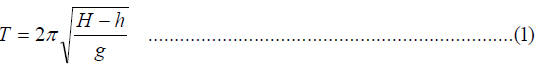
Which can be put in to the form

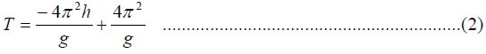
Note equation (2) is in the form of the equation of a straight line y = -mx + c,

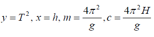
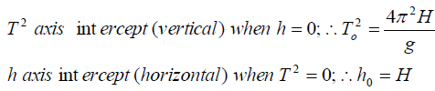
Equation (2) may be sketched by predicting the vertical,T_o² and horizontal h_o intercepts; if a graph of T² against h is to be drawn; as follows;

Sketch;

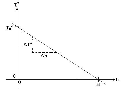
Since intercepts are needed, the axis must start at the origin, (0,0)

1.4.0 Deduction of experimental values

(i) Deducing the value of g. Since m is the slope of the equation, and in this cade it’s a negative, then

(ii) Deducing the value of H. Since the h-axis intercept,h₀ is equal to H, the we get its value directly from the intercept

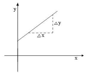
1.4.1 Determination of the slope

By definition, slope is the ration between the vertical change and horizontal change

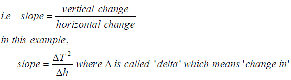
Its advisable to take large intervals of the slope .This minimizes the risk of too much approximations, and hence increases the accuracy of the results.

The calculated slope must be accompanied by the corresponding units of the physical quantities plotted.

1.5.0 Graph

The following points should be observed when drawing a graph. The graph should have:

(i) Title eg T² against h

(ii) Axes scales indicated ;e.g Vertical Scale: 1 cm : 0.2 s²,Horizontal Scale: 1cm : 5.0cm.

(iii) Axes drawn in sharp pencil and labeled in ink with quantities and units indicated.e.g Vertical axis T²(s) , Horizontal axis h (cm).

(iv) Correct and clear plotting of points.

(v) Line/Best line of fit / curve i.e The line or curve drawn should represent an estimated average of all practical graph points (vi) No calculations of any kind is allowed on the graph paper.

1.6.0 Errors Discussion:

At the end of each experiment report, error discussion should be presented. In this discussion ,the experimenter points out the physical factors which might have contributed to errors in the final result. For each error contribution mentioned a suggestion of how to minimize it has to be suggested.

COMMON SOURCES OF ERRORS IN MECHANICS AND PROPERTIES OF MATTER EXPERIMENT

Careless errors

1. Parallax in reading the scales of the physical quantities measuring instruments affect the accuracy of the recorded data Examples:

(i) Metre-rule used to measure length

(ii) Stop watch used to measure time

Precautions:

Readings should be taken in perpendicular position to the scale of the measuring instrument.

2. Time reaction in starting and stopping the stop-watch affect the accuracy of the recorded times Precautions:

Improve Care

A reference mark , e.g a chalk line should be used for observing crossing of oscillating body

3. Approximating reading from the scale of an instrument whose precision is poor (i.e scale not finely subdivided) Precautions:

A finely subdivided scale of the instrument should be used

Random errors

1.Air or wind resistance affect (damp) the oscillations of the system Precautions:

Minimize air resistance by closing windows and doors. Switch off ceiling fans

2 Frictional forces at the point of suspension damp the oscillations

Precautions:

Ensure rigid (firm) support at the point of suspension

Systematic errors

These arises due to the instrument used eg incorrect calibration of the instrument,zero adjustment etc.

Precaution

Inspect the instrument carefully.

Experiment No. M – 01

The aim of this experiment is to find the acceleration, g due to gravity by means of a simple pendulum.

Proceed as follows:

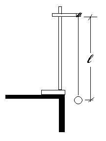
Fig. 1 .

Tie a thread to the pendulum bob provided.

Hang the pendulum bob so that the length, ℓ of the thread is 100 cm, as shown in Fig.1.

Pull the pendulum bob aside and release it so that it swings to and fro with small amplitude.

Find the time, t for 3 0 oscillations.

Repeat the experiment three times and find the average time, t. Find the period, T of the oscillations.

Record the results in a tabulated form.

Repeat this process for values of ℓ = 80 cm, 60 cm, 40 cm and 20 cm.

(a)Plot a graph of ℓ against T²

(b) Find the slope of the graph.

(c) Using the relation

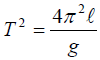
find the acceleration, g due to gravity. g

(d) Mention the sources of errors and their precautions in this experiment. (e) Further exercise: Use the same data to plot a graph of T² against ℓ and use it to find the acceleration, g due to gravity. Comment on your result.

Experiment No. M – 02

The aim of this experiment is to deduce a value of an unknown length fixed on a simple pendulum system.

Proceed as follows:

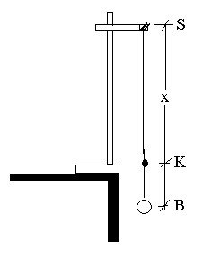
Fig. 2 .

Tie a knot, K such that KB is much shorter than the pendulum’s length, SB.

Suspend the pendulum as shown in Fig. 2

X, is the distance between the point of suspension S and the knot K on the string.

Adjust the string at its point of suspension so that X = 60 cm.

Swing the pendulum and measure the time, t for 20 oscillations of small amplitude.

Calculate the periodic time, T for one oscillation and hence determine, T².

Record the values of X, t, T, and T² in a tabular form. Repeat the above procedure for values of X = 40 cm, 30 cm, 20 cm and 10 cm.

(a) Plot a graph of T² (y-axis) against X. From the graph:

(i) Determine the values of the slope and the y-intercept of the graph.

(ii) Hence compute the ratio: P = (y-Intercept)/slope

(b) What is the physical significance of P.

(c) Use the value of the slope you have determined in (a) (i) to calculate a value of the acceleration, g due to gravity.

Experiment No. M-03

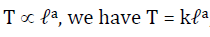
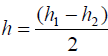
The aim of this experiment is to determine the acceleration, g due to gravity and an unknown height, H using a simple pendulum.

Proceed as follows:

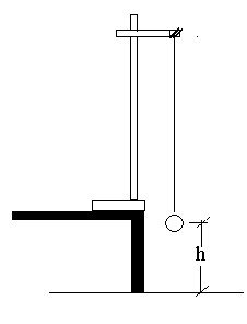
Fig. 3 .

You are provided with a piece of thread and a pendulum bob.

Tie one end of the thread to the pendulum bob and fix the other end to the point of suspension, S so that the pendulum bob is at the height, h of about 5 cm from the floor as shown in Fig. 3.

Displace the pendulum through a small angle to one side and let it oscillate. Record the time t for 30 oscillations and hence find the period T for one complete oscillation.

Increase the height, h of the bob above the floor by about 5 cm and repeat the above procedure. Do this for four other values of h, each time increasing h by about 5 cm.

Tabulate your results.

If the period, T is related to the height, h by the relation:

(a) Plot a graph of T² against h.

(b) From your graph, determine:

(i) The slope and hence the value of the acceleration g, due to gravity.

(ii) A value of H from the h – axis intercept.

(c) What is the physical significance of H?

Further exercise: If you were to plot a graph of h against T², what answers would you have for part (b) above?

Experiment No. M – 04

In this experiment you are required to find the relationship between the length, l of a simple pendulum and its period, T (the time for one oscillation).

Proceed as follows:-

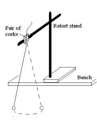
Fig. 4 .

Suspend a simple pendulum of length 140 cm, as shown in Fig.4.

Displace the pendulum through a small angle so as to make it swing in a vertical plane parallel to the edge of the bench (or table).

Determine the time needed for 20 oscillations of the pendulum.

Now reduce the length of the pendulum by 20 cm and again find the time for 20 oscillations.

Continue reducing the length of the pendulum by 20 cm each time, and obtain a total of six readings.

(Don’t repeat any reading of the time taken for 20 oscillations so as to find an average time to be recorded)

Record your readings in a table as shown below:-

Length of pendulum,ℓ(cm)	Log10ℓ	Time for 20 oscillations (s)	Periodic time, T(s)	Log10T

Assuming that

and taking logarithms to base ten we obtain:

Log₁₀T = a log₁₀ℓ + log₁₀k

(i) Plot a graph of log₁₀T (vertical axis) against log₁₀ℓ (horizontal axis). Hence determine the values of “a” and ‘k’ (each correct to one decimal place).

(ii) From your answer in (i) above, write down the values of ‘a’ and then, ‘k’ each in the form b/c where b and c are integers (i.e. whole numbers).

(iii) From the assumption and your answer in (ii) deduce the form of the equation governing the motion of the simple pendulum.

Experiment No. M – 05

The aim of this experiment is to determine the acceleration, g due to gravity at your local area, and a constant T_c for the ruler provided.

Proceed as follows:-

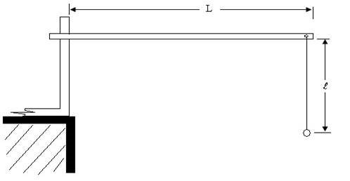
Fig. 5 .

(a) (i) Using a vice or clamp, fix the metre-rule on one leg of a bench (or stool) as shown in Fig 5. The flat part of the metre-rule should be vertical and the projection L from the fixed end should be 80 cm.

(ii) By means of the string given, suspend the pendulum bob from the hole through the metre-rule as illustrated in Fig. 5.

(b) (i) Starting with ℓ = 80 cm, displace the bob through a small angle along

the direction of the length of the ruler and then release it so that it performs small-amplitude oscillations.

Record the time, t for 20 complete oscillations and hence the period, T for one oscillation.

(ii) Without altering L, repeat (b) (i) above for the following values of ℓ in turn: 70 cm, 60 cm, 50 cm, and 20 cm.

(c) Given that:

Plot a graph of T² against ℓ, and use it to determine: (i) The acceleration due to gravity, g at your local area, and (ii) The constant, T_c.

(d) What is the physical significance of the constant T_c in your experiment?

(e) State any sources of errors involved and precautions taken in this experiment.

Experiment No. M - 06

The aim of this experiment is to determine the gravitational field intensity, g using a spiral spring.

Proceed with the experiment as follows:

Fig. 6

(a) (i) Set up the apparatus as illustrated in Fig. 6 above so that a 150 g, wooden block hangs vertically from the lower end of the spring.

(ii) Measure the distance h between the floor and the lower end of the spring.

(iii) Now pull the wooden block downwards through a short distance and then release it thus allowing it to perform simple harmonic motion.

(iv) Measure the time t taken by 20 complete oscillations and hence determine the corresponding period, T of the motion.

(v) Calculate the corresponding value of T².

(b) Repeat the procedure described in (a) above five times, each time using a different wooden block. The blocks increase in mass by steps of 50 g.

Tabulate your results in a tabular form as shown below:

h (cm)

m (g)

t (s) for 20 oscillations

T (s)

T2 (s2)

(i) Plot a graph of h against T² (whose values are recorded in (i) and find its gradient.

(ii) Determine the gravitational field intensity, g given that both h and T are related through the equation:

Where: H is a constant.

(iii) Determine from the graph a value of H.

(iv) What is the physical significance of H?

Experiment No. M – 07

The aim of this experiment is to determine the spring constant, k and the effective mass, S of the spiral spring provided.

Proceed as follows:

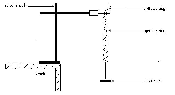Fig. 7 .

(a) Suspend the spiral spring with its scale pan from the support A as shown in Fig. 7

(b) Load it with mass, m =100 g. Pull the scale pan slightly below the equilibrium position and release it so that the system executes vertical oscillations of small amplitude.

(c) Record the time for 20 vertical oscillations and determine the period, T.

(d) Repeat this procedure with five other different masses in steps of 50 g.

(e) If the period, T and the spring constant, k are related by an expression of the form:

(i) Use the given expression to plot a graph of T² against m.

(ii) Use your graph to determine the quantities k and S.

Experiment No. M-08

The aim of this experiment is to determine the earth’s gravitational intensity, g and the effective mass s of the spiral spring.

Proceed as follows:

Fig. 8 .

Suspend the spiral spring, so with its scale pan, P from a rigid support. Attach a light pointer, R to the spring. Set up a fixed vertical metre rule, C besides the spring (Fig. 12). Record the initial reading of the pointer and then add suitable weights, m noting the reading of the pointer each time. Obtain about six readings. Tabulate your results.

If the extension, x of the spring is related to the added weights m by: g g

Where k is the elastic constant of the spring, (k=13.0Nm-¹) plot a graph of x against m.

Use the given relation and your graph to determine:

(a) A value of g, in Newton’s per kilogramme, (b) A value for S in kilogrammes.

Experiment No. M – 09

The aim of this experiment is to determine the value of the spring constant, k of the helical spring provided.

Proceed as follows:

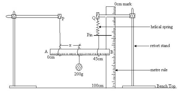Fig. 9 .

(a) Set up the apparatus as shown in Fig. 9 without the 200 g mass, where:

(i) Points of suspension P and Q are 40 cm apart,

(ii) Loops 1 and 2 are at 5 cm and 45 cm marks, respectively,

(iii) The pin is attached to the lower end of the helical spring using plasticine,

(iv) A short string connects the lower end of the spring to loop 2.

(v) Loop 1 is attached to P with a long string, and

(vi) The half metre-rule, AB is horizontal such that the edges A and B

are at equal heights from the bench. This is achieved by adjusting

the length of the string suspended from P.

(b) Measure the height of the pin from the bench. Record it as Y₀.

(c) (i) Suspend the 200 g mass provided, at loop 3. Use a short string.

(ii) Adjust loop 3 so that the 200 g mass hangs at the 40 cm mark. i.e.

X=35cm.

(iii) Adjust the string length from P such that AB is horizontal again.

(iv) Record the distance X, between the loops 1 and 3 and measure the

corresponding height, Y of the pin from the bench. Hence determine Y-Y₀.

(v) Repeat steps (c ) (ii), (iii) and (iv) for values of X = 30, 25. 20, 15

and 10 cm, and record the corresponding values of Y and Y-Y₀.

(d) Plot a graph of Y-Y₀ (y-axis) against X.

(e) (i) Determine the slope, S of the graph and hence

(ii) Calculate the value of k given that:

Experiment No. M – 10

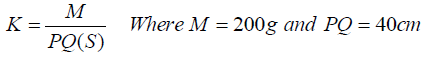
The aim of this experiment is to determine the acceleration, g due to gravity by means of oscillations and extensions of masses on a spiral spring.

Proceed as follows:

(a) Set up the apparatus as shown in Fig. 10 (a). Put on the scale pan a mass, m say, 100 gm and record the time T taken to complete 10 oscillations.

Repeat the procedure for at least four other masses, and for each record the corresponding time T for 10 oscillations. Record the values of m and T.

(b) Move the vertical metre-rule scale and the retort stand (Fig. 10 (b) towards the spring so that the pointer on the spring can be used to record readings on the metre-rule (whose 100 cm-mark should be at the bottom)

(c) With a mass m₁, say 50 gm record the corresponding reading of the pointer as r₁ on a vertical metre-rule. Repeat this procedure with another mass, m₂ and record the corresponding pointer reading r₂.

(d) Plot a graph of T² (vertical axis) against mass, m (horizontal axis). From your graph determine the slope, S.

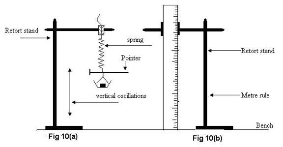
(e) Calculate the acceleration due to gravity, g given that:

(f) State any sources of errors and precautions taken in this experiment.

Experiment No. M - 11

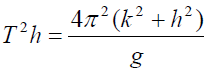
The aim of this experiment is to determine the gravitational intensity, g and the radius of gyration, k of the given block of wood.

Proceed as follows:

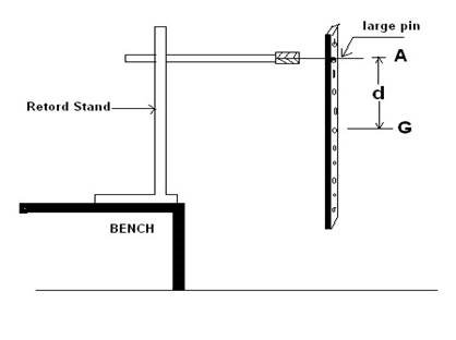
Fig. 11 .

(a) (i) Set up the apparatus as shown in Fig. 11. The length AG is the distance, d measured from the center of gravity G of the block.

Suspend the block of wood from a hole made at one end.

(ii) With a stop watch, take the time t for 10 small complete oscillations of the block, and hence determine the periodic time, T.

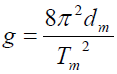
(iii) Repeat the above procedures with 6 other values of d, and in each case, record the corresponding time, t and hence the periodic time T. Make a table that includes the following headings:- d, t, T, T², T²d and d²

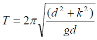
(b) Given that the periodic time, T is given by:-

Where k is the radius of gyration of the block of wood about the center of gravity, then:-

(c) Plot a graph of T²d (y-axis) against d². (Both axes of the graph should start at the origin).

(d) Use your graph and the equation above to determine:

(i) The gravitational intensity, g (ii) (iii) The radius of gyration, k

Experiment No. M – 12

The aim of this experiment is to determine the value of the acceleration, g due to gravity by means of a compound pendulum.

Proceed as follows:

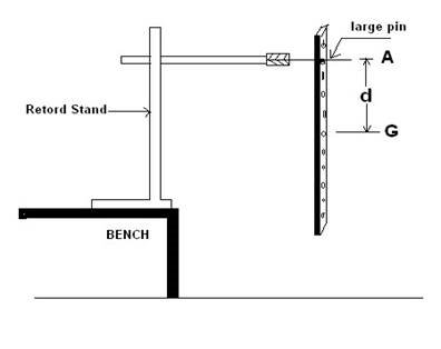
Fig. 12 .

(a) Set up the apparatus shown in Fig.12, where the wooden bar is suspended by a nail or thick pin through a hole nearest the line marked G. Use the pieces of wood or split corks to hold the nail or thick pin in the clamp. The holes in the wooden bar are drilled at 5 cm intervals.

(b) Displace the bar through a small angle and find the time for 20 complete oscillations. Change the point of suspension, so that the distance, h is 10 cm as measured from G and again find the time for 20 complete oscillations.

Continue with this procedures until you arrive at the hole nearest to the end marked A.

Tabulate your results and include a column for the periodic time, T.

(c) Plot a graph of T against h. The graph is a smooth curve.

(d) Draw a horizontal tangent on the curve and use this to read the coordinates of the minimum point on your graph.

Record the coordinates as (h_m,T_m).

(e) Calculate the value of the acceleration due to gravity, g using the relation:

Give your answer in SI units.

(f) (i) What would have been the periodic time, t if a hole were drilled at G and used as a point of suspension?

(ii) What would you expect to happen if the bar were displaced through a small angle when suspended through a hole at G?

Experiment No. M-13

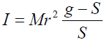
The aim of this experiment is to determine the moment of inertia, I of a wooden bar acting as a bifilar pendulum.

Proceed as follows:-

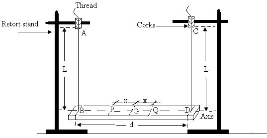Fig. 13 .

(a) Locate the center of gravity, G, of the wooden bar by balancing it on a knife edge. Draw the horizontal axis of the bar through G.

(b) Using the pieces of cork and pieces of thread provided, suspend the wooden bar as shown in Fig. 13, such that L = d = AB = CD = 100 cm. Make sure that the threads are vertical and parallel.

(c) Make adjustments so that the wooden bar is perfectly horizontal, and the length, d is symmetrical about G. (i.e. GB = GD).

(d) Measure distance x = 5 cm from each side of G and let the arbitrary distance positions be P and Q as shown in Fig. 13.

(e) Place a 100 g mass at P and another 100 g at Q. Tie them firmly on the wooden bar using the light rubber bands provided. Set the wooden bar oscillating about a vertical axis through G. Record the time for 10 complete oscillations and calculate the corresponding periodic time, T.

(f) Move the 100 g masses along the horizontal axis about the center of mass of the wooden bar by increasing the distance x intervals of 5 cm from each side of G. At each position of the masses, measure the time, t for 10 complete oscillations and determine the corresponding periodic time, T. Tabulate your results.

(g) Plot a graph of T² (vertical axis) against x² (horizontal axis).

(h) Given that:

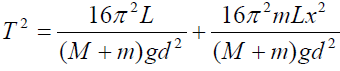
Where L and d are expressed in S.I units, g=9.81 ms^-2 and m = 0.2 kg, use your graph to determine M and I ,What does M represent?

(i) Mention any precaution(s) that you took in performing this experiment

Experiment No. M 14

The aim of this experiment is to investigate the relationship concerning the periodic time, T and the separation, X of a bifilar pendulum.

Proceed as follows:

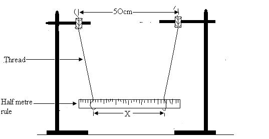Fig. 14 .

(a) Suspended the half metre-rule using threads of about 80 cm each from the top of the clamps, which should be about 50 cm apart as shown in Fig.14. The lower ends of the threads are looped to the rule at equal distances from the mid-point of the rule. Record the separation X between the loops.

(b) Set the pendulum (the rule) swinging horizontally by displacing the ends of the rule in the opposite direction through a small angle.

Determine the time, t needed for 10 such oscillations of the pendulum.

Keeping the lengths of the threads fixed and the distance between the clamps unchanged; reduce the separation, X between the loops making sure that the loops are equidistant from the mid-point of the rule.

Repeat the oscillations and determine the time, t for 10 oscillations.

(d) Continue this way so that at least six different observations of t corresponding to X are obtained.

Record your observations neatly, including values of the periodic time, T (time for one oscillation), log₁₀T and log₁₀X.

(e) Assuming that T ∝ X^-n, we have T = kX^-n where k is a constant and n is a fraction.

Taking logarithms, we obtain:

Log₁₀T = - nlog₁₀X + log₁₀k

(i) Plot a graph of log₁₀T (vertical axis) against log₁₀X (start your axes at (0,0)).

Hence determine the values n and k, each correct to one decimal place.

(ii) Rounding the values of k and n, deduce the form of equation concerning the relationship between the periodic time, T and the separation, X.

Experiment No. M 15

The aim of this experiment is to determine the radius of gyration, k of the square sheet of cardboard provided and the acceleration, g due to gravity.

Proceed as follows:

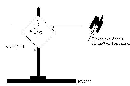Fig. 15 .

(a) Using the weighted string (or plumbline), locate the centre of gravity G of the card-board provided. Briefly, with the aid of sketch diagrams, explain how you locate the centre of gravity G.

(b) Draw a line from the centre of gravity G to any of the four corners of the card-board. Measure a distance of 2 cm from G along this line and make a hole at this point. Make five other holes along the line such that all the holes are at distances of 2 cm from each other.

Set up the apparatus as shown in Fig. 15 above.

Suspend the card-board from a hole nearest to the centre of gravity G. Record the distance, d which is the distance of the hole from G. Using the stop-watch provided, obtain the time for 10 small complete oscillations of the card-board; and hence calculate the periodic time, T.

Repeat the above procedure with 5 other values of d and obtain the corresponding values of T.

(d) Given that:

Plot a graph of T²d against d², with both axes starting at the origin.

Use the graph and the equation to determine:

(i) The radius of gyration, k of the square sheet of card-board.

(ii) The acceleration, g due to gravity

(e) Mention any two random errors and any two systematic errors in this experiment. Explain the precautions necessary for each source of error you mention.

Experiment No. M 16

The aim of this experiment is to determine the acceleration due to gravity, g and radius of gyration, k of the triangular sheet of card-board provided.

Proceed as follows:

(a) Using the weighted string (or plumbline) provided, locate the center of gravity G of the triangular sheet of card-board. Briefly, with the aid of a sketch diagram, explain how you obtain G.

(b) Draw a line joining G and the farthest angle (Apex) A of the card-board. Measure a distance 2 cm from G, along the line GA. Make a hole at this point. Make five other holes along GA at distances 2 cm from each other.

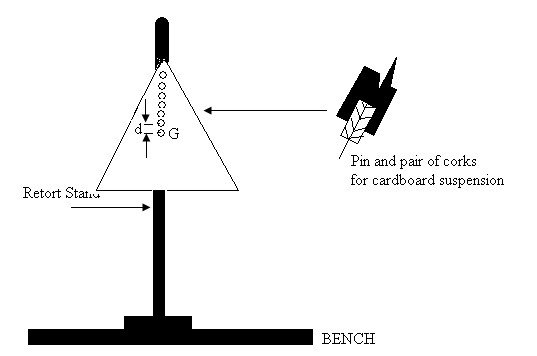Fig. 16 .

Set up the apparatus as shown in Fig. 16 above. The pin should be clamped tightly between the two pieces of corks. Suspend the triangular card-board from a hole nearest the center of Gravity G. Record h, which is the distance of the point of suspension from G.

With the stop watch provided, obtain the time, t for 10 small complete oscillations of the card-board and hence determine the periodic time, T.

Repeat the above procedure with five other values of h to obtain corresponding values of t and T.

(d) Plot a graph of h² against T²h, with the origin at (0,0)

Determine, with the aid of your graph,

(i) The acceleration, g, due to gravity, and (ii) The radius of gyration, k.

Experiment No. M-17

The aim of this experiment is to determine the radius of gyration of a solid spherical ball about an axis through its center.

Proceed as follows:

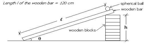Fig. 17 .

(a) (i) Place ten (10) wooden blocks of dimensions 5 cm x 3 cm x 0.9 cm one

on top of the other so that the total height h is 9 cm.

(ii) Place a wooden bar of length 120 cm so that is makes an inclination as shown in Fig. 17. The wooden bar should have a track made at its center to enable the ball to roll.

(iii) With L = 110 cm, start the ball from rest at M and measure the time, t taken to reach the bottom at N.

Repeat this three times.

(b) Repeat the procedure in (a) above by removing six (6) blocks one at a time, in order to obtain a total of six readings.

Tabulate your results as follows:

Height h(cm)

t1 (s)

t2 (s)

t3 (s)

Average Time, t (s)

t2 (s2)

Sin =h/L

Acceleration A=2L/t2(cm/s2)

(c) Using a micrometer screw gauge, measure the mean diameter, d of the ball and hence calculate its mean radius, r in centimetres.

(d) Plot a graph of acceleration, A against Sin (horizontal axis).

(e) Calculate the slope S of your graph.

(f) Calculate the radius of gyration, k of the ball given that:-

Where: M is the mass of the ball and g = 9.81 ms^-2

(g) State any two sources of errors in this experiment.

Experiment No. pM – 01

The aim of this experiment is to determine the mass of a loaded metre rule by balancing it on a knife-edge. Requirements

S/No	ITEM	SPECIFICATIONS	QUANTITY/ STUDENT
1.	Masses	100 g	2
2.	Metre-rule	Millimetre scale	1
3.	Knife edge	wooden	1
4.	Wooden block	20 cm height	1
5.	Cotton string	50 cm -Inelastic	set
6.	Graph paper	Metric type	1

C: Objectives

The student should be able to:

(a) Assemble the apparatus as indicated or described in the instructions.

(b) Take measurements and record data in a tabular form.

(c) Plot a graph of y against x (with both axes starting at the origin).

(d) Determine the slope of the graph.

(e) Determine the y-axis intercept.

(f) Use the given relation to calculate the mass of the metre-rule.

(g) Discuss sources of random and systematic (persistent) errors related to the experiment and suggest precautions/ways/methods of minimizing them.

Theory

Graph of y against x

Given:

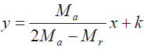
This is an equation of a straight line.

Proceed as follows:-

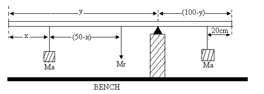Fig. 18 .

(a) By means of a strong elastic band, securely fix 100 g brass weight underneath the 80 cm mark of a metre-rule, the flat base of the weight being in contact with the rule. Let the mass of the rule be M_r

(b) Attach a small loop of thread to the second 100 g mass, (M_a). Suspend this weight at a distance x from the zero end of the rule. Using the values of x indicated on the table below, balance the rule on the knife-edge and note the distance y of the knife-edge from the zero end of the rule.

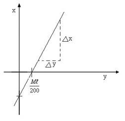
(c) Plot the graph of y (vertical axis) against x (horizontal axis).

(d) Find the gradient of the graph and the intercept on the y-axis.

(e) Given that, your graph obeys the equation:

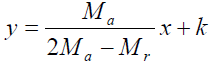
Deduce the value of M_r

Table of results

x (cm)	15	20	30	40	50	60
y (cm)

Experiment No. pM-02

In this experiment you are to determine the mass of a given wooden rectangular rod and that of another object labeled ‘m’.

Requirements

S/No	ITEM	SPECIFICATIONS	QUANTITY/ STUDENT
1.	Wooden rectangular rod (or a metrerule)	With a hole at the centre	1
2.	Mass	200 g
3.	Unknown Mass, m	About 100g	1
4.	Metre-rule	Millimetre scale	1
5.	Retort stand with accesories		1
6.	Knife edge	wooden	1
7.	Cotton string	50 cm -Inelastic	set
8.	Graph paper	Metric type	1

Objectives

The student should be able to:

(a) Assemble the apparatus as indicated or described in the instructions.

(b) Take measurements and record data in a tabular form.

(c) Plot a graph of x against y (with both axes starting at the origin).

(d) Determine the slope of the graph.

(e) Determine the y-axis intercept.

(f) Use the given relation to deduce the mass, M of the wooden rectangular rod.

(g) Use the given relation to deduce the unknown mass, m

(h) Discuss sources of random and systematic (persistent) errors related to

the experiment and suggest precautions/ways/methods of minimizing them.

D: Theory

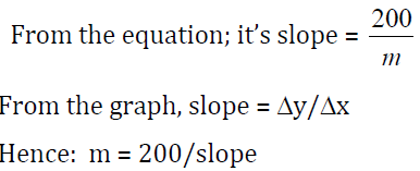
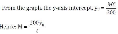
Graph of x against y

Given:

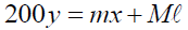
Make x the subject of the formula:

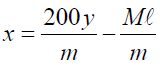
Where: m is the mass of the unknown mass and M is the mass of the rectangular rod.

This is an equation of a straight line.

(a)

(b)

Proceed as follows:-

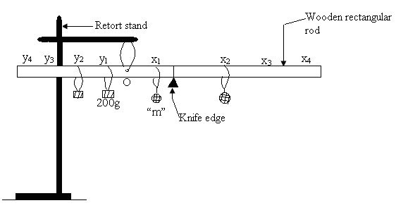
(a) Suspend the given wooden rectangular rod to a retort stand with a thread through a hole marked ‘O’. (Note that O is not the center of gravity of the rod)

Suspend the given standard mass of 200 g on the shorter arm and the unknown mass labeled ‘m’ on the longer arm of the rod; mark the position of the thread suspending the known mass with pencil and label it y₁ (see Fig. 2).

The position of the unknown mass where the rod is balanced in horizontal equilibrium is also marked with pencil along the position of thread and labeled x₁.

(b) Move the position of the known mass about 5cm from the first position away from the pivot ‘O’ and mark this position y₂. Balance it with the unknown mass ‘m’ by moving it until the level is again in horizontal equilibrium. This position of the unknown mass is labeled x₂.

(c) Repeat the same procedure while in each step, the known mass is moved through distances of about 5 cm, away from the previous position. Mark these positions as y₃,y₄,y₅,y₆, etc and their corresponding positions x₃,x₄,x₅,x₆, etc of the unknown mass ‘m’ which sets the level in horizontal equilibrium at each stage.

(d) Remove the wooden rod from the point of suspension and take away the two masses.Measure the distances Ox₁, Ox₂, Ox₃, etc and their corresponding distances Oy₁, Oy₂, Oy₃, etc and tabulate them as x and y values respectively.

(e) Without anything on the wooden rod, balance it on a knife edge to determine point ‘C’ where it balances freely in horizontal equilibrium.

Measure and record distance OC = L.

(f) When the rod is in equilibrium (i.e balanced), it is governed by the equation:

Where: m is the mass of the unknown mass ‘m’ and M is the mass of the given wooden rectangular rod.

Plot a graph of x against y and use it to determine:-

(i) The values of m and M.

(ii) State any sources of errors in this experiment.

Table of results

y(cm)	5	10	15	20	25	30
x(cm)

Experiment No. pM-03

The aim of this experiment is to determine the density of wood.

Requirements

S/No	ITEM	SPECIFICATIONS	QUANTITY/ STUDENT
1.	Mass	100 g	1
2.	Wooden Bar	e.g Metre-rule	1
3.	Knife edge	wooden	1
4.	Wooden block	20 cm height	1
5.	Vernier Calipers	Millimetre scale	1
6.	Cotton string	50 cm -Inelastic	set
7.	Graph paper	Metric type	1

Objectives

The student should be able to:

(a) Assemble the apparatus as indicated or described in the instructions.

(b) Take measurements and record data in a tabular form.

(c) Plot a graph of Y against X.

(d) Determine the gradient, G of the graph.

(e) Deduce the value of the mass of the wooden bar using the given relation.

(f) Use the vernier calipers to measure width and thickness of the wooden bar.

(g) Use the given relation to calculate the density of the wooden bar.

(h) Discuss sources of random and systematic (persistent) errors related to the experiment and suggest precautions/ways/methods of minimizing them.

Theory

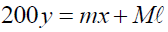
Graph of Y against X

The center of gravity, C is located as described.

The gradient, G is related to the mass, M of the wooden bar by:

Where: ℓ, w and t are the length, width and thickness of the wooden bar. w and t are measured using vernier calipers.

Proceed as follows:

You are provided with a wooden bar, a knife edge and a 100 g mass

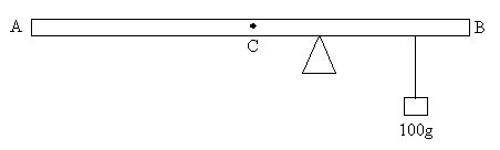
(a) Locate the center of gravity C of the wooden bar by balancing it freely about the knife-edge.

(b) Suspend the 100 g mass of the wooden bar at 10 cm from C and adjust the position of the knife edge to get a balance, as shown in Fig. 3.

(c) Record the distance of center of gravity C from the knife edge as Y and distance between the knife edge and 100 g mass as X.

(d) Repeat procedures (b) and (c) above, by increasing the distance of the 100 g mass to 20 cm, 30 cm, 40 cm, 50 cm, 60 cm, respectively from the center of gravity C. Tabulate your results

(e) Draw a graph of Y against X and calculate its gradient, G. Calculate the mass,

M of the wooden bar, given that:

Gradient,

(f) Measure the length, L with, w and thickness, t of the wooden bar and hence calculate the density of wood given that:

Density of wood,

Table of results

X(cm)	10	20	30	40	50	60
Y(cm)

Experiment No. pM-04

The aim of this experiment is to determine the density of the material of wire W.

Time: 2 Hours

Requirements

S/No	ITEM	SPECIFICATIONS	QUANTITY/ STUDENT
1.	Wire W	Copper SWG 24	100cm
2.	30-cm ruler (Millimetre scale)	With a hole at center	1
3.	Weights	Set of 0.5 – 3.0 g	1
4.	Weight	5 g	1
5.	Retort stand	With accessories	1
6.	Large pin	Optical pin	1
7.	A pair of corks	to grip pin	1
8.	Micrometer screw gauge	Millimetre scale	1
9.	Pan	Made of the inside of a match box	1
10.	Wire	Thin (for loop)	15 cm
11.	Cotton string	50 cm -Inelastic	set
12.	Wire cutter	Prize	1
13.	Graph paper	Metric type	1

Objectives

The student should be able to:

(a) Assemble the apparatus as indicated or described in the instructions.

(b) Take measurements and record data in a tabular form.

(c) Plot a graph of y against m.

(d) Determine the slope, S₁ of the graph.

(e) Plot a graph of y against L.

(f) Determine the slope, S₂.

(g) Measure the diameter of wire W using a micrometer screw gauge.

(h) Calculate k, the mass per unit length using the given relation.

(i) Calculate the density of the material of the wire W.

(j) Discuss sources of random and systematic (persistent) errors related to the experiment and suggest precautions/ways/methods of minimizing them.

Theory

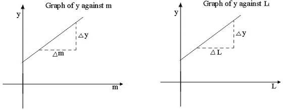
From the graph of y against m:

Slope,

From the graph of y against L:

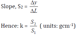
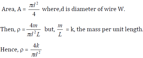
Since, density,

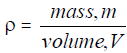
where,volume, V = cross-sectional area, A x length, volume,V

Proceed as follows :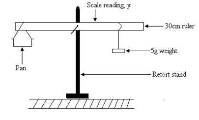

You are provided with a 30 cm ruler with a hole in the middle. Hang the ruler with the pin provided.

Hang the weighing pan, made of the inside of a match box, near the zero cm mark.

Balance this by hanging a 5 g mass in the loop of wire attached to the ruler. Use the thread provided. Slide the loop until the ruler is balanced. Note the scale reading y where the loop of wire rests. This reading corresponds to zero mass in the pan. Denote it by y_o.

(a) Add a ½ g mass in the pan and move the 5 g weight until the ruler is balanced. Observe the new value of y and record it. Continue adding weights to the pan, ½ g at a time, and record the values of y corresponding to the mass, m in the pan. Plot a graph of y (y-axis) against m and record its slope S₁.

(b) Again starting with y_o, add to the weighing pan about 20 cm of the wire labeled W. Again balance the ruler and determine the scale reading y. Repeat this for at least 4 more values of L (where L is the total length of the wire in the pan) and record the corresponding values of y. Plot a graph of y(y-axis) against L and record the slope S₂.

(c) Measure the diameter of the wire W and calculate its cross sectional area, A.

(d) If the mass per unit length, k of the wire W is given by:

Determine K and hence calculate the density of the material of the material of the wire W.

Table of results

Table 1

m (g)	0.5	1.0	1.5	2.0	2.5	3.0
y (cm)

Table 2

L (cm)	20	40	60	80	100	20
y (cm)

Experiment No. pM – 05

The aim of this experiment is to determine the density of the material of which the given test tube is made.

Proceed as follows:

(a) Find the average circumference, A_c of the test tube labeled A by wrapping 10 turns of the given wire labeled WW in a closely round spiral at three different places on the test tube.

(i) Determine the radius, WW_r of the wire using the micrometer screw gauge provided.

(ii) Find the average length, WW₁ of one turn of the spiral.

(iii) Calculate the circumference, A_c of the test tube using the formula:

A_c = WW₁ – 6.3WW_r

(iv) Calculate the mean external area of cross-section, A_e of the test tube given by the formula:

(b) Determine the internal area of cross-section, A_i of the test-tube by volumetric method as follows:

(i) Clamp the test-tube vertically with its base resting on a flat surface.

(ii) Fill the given measuring cylinder with liquid, LL to the 50 cm³ mark.

(iii) Pour about 2.0 cm³ of liquid LL from the measuring cylinder into the test tube A.

(iv) Record the reading, V of the liquid LL from the measuring cylinder and the height, h of the liquid LL level above the base of the test tube.

Repeat the experiment, each time adding about 2.0 cm³ more of liquid LL to the test tube, without pouring out the initial liquid, to obtain six (6) more readings.

1. Tabulate h, V and W, where W is the volume of liquid LL poured into the test-tube.

2. Plot a graph of W against h.

3. Determine the gradient (slope), A_i (of the line) which is the internal area of cross-section of the test tube.

(c) Measure the length, L of the test tube, A and calculate the volume VV of the material of which the test tube is made from the formula:

VV = L(A_e – A_i).

(d) Weigh test-tube A to find its mass, m in grams.

Hence determine the density of the material of which the test tube is made.

Experiment No. pM-06

In this experiment you are required to determine the density of liquid L₂ relative to that of liquid L₁ and the mass, M of the metre-rule provided.

Proceed as follows:

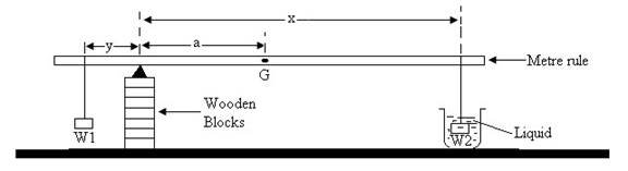Fig. 23 .

(a) Locate and mark the center of gravity G of the metre rule.

(b) Set up the apparatus as illustrated in Fig. 6, where: a =50 cm, W₁ and W₂ are brass weights of mass 50 g and 20 g, respectively.

(c) With W₂ totally immersed in liquid L₁ and x = 10 cm, balance the metre-rule on the knife edge by adjusting the position of W₁. Read and record the distance, y. Repeat the procedure for x = 20 cm, 30 cm, 40 cm, 50 cm and 54 cm. Tabulate the values of x and y.

(d) Replace liquid L₁ by liquid L₂ and then repeat the procedure outlined in (c) above.

(e) Plot a graph of y against x using the table obtained in (c).

(i) Read and record C₁ the value of y when x = 0. Calculate 10C₁, which is equal to the mass of the metre-rule.

(ii) Find the slope, S₁ of the graph.

(iii)Find the value of λ ₁ given that λ ₁ = 0.4 - S₁

(f) Plot a graph of y against x using the table obtained in (d).

(i) Find the slope S₂ of this graph.

(ii) Find the value of λ ₂ given that λ ₂ = 0.4 - S₂.

(iii) Evaluate the ratio λ ₂/λ ₁ which is equal to the density of liquid L₂ relative to that of liquid L₁.

(g) Discuss sources of errors in this experiment.

Experiment No. pM – 07

The aim of this experiment is to determine the density of motor oil L₀ relative to liquid L₁ and the density of the material of the metre-rule provided.

Proceed as follows:

(a) Locate and mark the center of gravity G of the metre-rule. Measure the width and thickness of the rule (use vernier calipers).

(b) Assemble the apparatus as shown in Fig. 7 below.

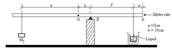Fig. 24 .

(c) Fix the knife edge E, 10 cm from G towards A and the 100 g (M₁) 5 cm from the end marked A.

(d) With M₁ totally immersed in liquid L₁, adjust the position of the 50 g (M₂) until the rule is balanced horizontally. Record the positions of M₁, M₂, and distances x and y.

(e) Move M₁ five centimeters towards E and repeat the experiment. Record the new positions of M₁ and M₂ and the distances x and y as in (d).

(f) Do this experiment, each time moving M₁ by 5 cm towards E to obtain total of five sets of readings. Tabulate your results.

(g) Replace liquid L₁ by the motor oil L₀ and repeat the procedure outlined in (d), (e), and (f) above.

(h) Plot graphs of y against x for liquid L₁ and motor oil L₀ (use different graph papers).

(i) Find the slope S₁ for liquid L₁

(ii) Find the slope S₀ for motor oil L₀

(iii) Read the y – intercepts C₁ and C₀ for the two graphs.

(i) Find the value U₁ and U_o given that:

(j) Calculate the density of motor oil L₀ relative to liquid L₁ , given that:

(k) Determine the mass M of the metre rule given that:-

Hence determine the density of the wooden material of the rule.

Experiment No. pM-08

The aim of this experiment is to determine the relative density of the liquid provided.

Proceed as follows:

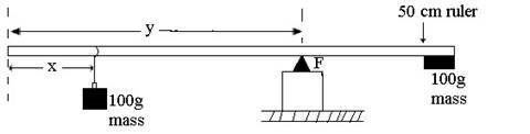
Fig. 25 .

First determine the mass M_r of the rule as follows:

Hang the 100 g mass at the 4 cm mark and balance the ruler by adjusting its position of support on the knife-edge F. Measure and record the value of X and Y as shown in

Fig. 8.

Let these values be X₁ and Y₁ respectively. Next hang the 100 g mass at the 20 cm mark of the ruler, and again balance the ruler by adjusting its position of support on the knife edge. Measure and record the new values of X and Y.

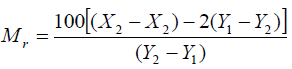
Let these values be X₂ and Y₂, respectively Calculate M_r from the equation:

(a) With the 100 g mass at the 4 cm mark of the ruler and submerged fully in water contained in the beaker provided, balance the ruler again and determine the corresponding value of Y. Repeat this procedure taking 5 readings of X and Y for values of X varying between 4 and 20 cm. Plot a graph of Y(y-axis) against X. Determine its slope S₁

(b) Repeat the procedure in(a), but this time submerging the 100 g mass in the liquid L. Record 5 readings of X and Y and plot a graph of Y against X on a separate graph. Determine the slope S₂ of the graph.

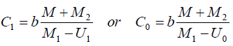
(c) If M_w and M_L represent the apparent mass of the 100 g mass in water and in L, respectively,

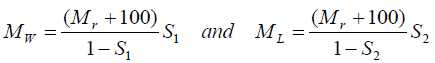
Using the above equations, determine:

(i) M_w and M_L and thus

(ii) The relative density of the liquid L

Experiment No. pM-09

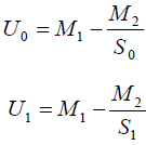
The aim of this experiment is to determine the relative density of the motor oil provided.

Proceed as follows:

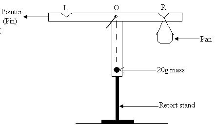
Fig. 26 (a) .

(a) Hang the wooden T provided with a pin though the hole at 0.

On the lower end of the T fix a 20 g mass using a little plasticine.

On the left side L attach a large pin with some plasticine.

This pin acts as a pointer.

With the help of plasticine, balance the T so that its arm LR is approximately horizontal.

(b) First determine the height, h₀ of the pointer from the table. Adding two grammes to the pan, at a time, determine the corresponding heights, H of the pointer from the table.

Record your observations and plot a graph of (H – h₀) against the mass, m in the pan.

(Note that the graph is not a straight line).

Fig. 26 (b) .

(c) Take two 100 g masses and hang them with short pieces of thread on each side.

Adding plasticine, bring LR to an approximately horizontal position.

Measure again the new height h₀.

Now fill the beaker provided with water and raise the beaker so that the left hand mass is fully submerged in water.

Measure the new height H_w of the pointer.

From the graph determine the corresponding up thrust.

(d) Repeat the procedure in (c), but this time, submerge the left hand 100 g mass in the beaker containing the motor oil.

Measure the corresponding new height H₀.

From the graph determine the corresponding up thrust.

(e) From your observation in (c) and (d), determine the relative density of the motor oil under investigation. Give the theory by which you determine the answer.

Physics Practical

Experiment No. pM-10

The aim of this experiment is to determine the density of material of wire labeled X.

Proceed as follows:-

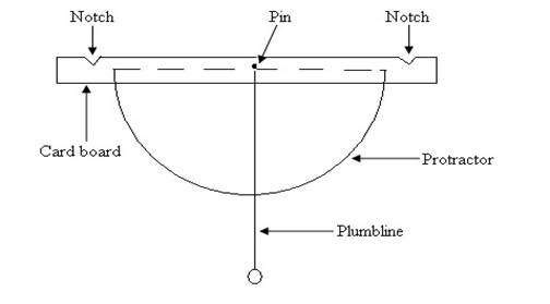
Fig 27 .

(a) (i) Determine the mass per metre of the wire labeled “A”.

The supervisor will give you the value of the mass of the wire. (ii) Cut a pair of notches on the cardboard strip and then attach it to the protractor

with sellotape. The notches should be cut so that their tips are 10.0 cm from

the pivot and on the same straight line passing through the pivot. Make a simple balance as shown in Fig. 27.

The balance should be adjusted so that the 0^o- 0^o line is horizontal. A small pellet of plasticine may be used for this purpose.

(b) Suspend the wire A on one of the notches and record the deflection _A of the balance it produces. Cut off a small length of the wire A and measure the length,

L of the remaining portion. As before, suspend the length, L on the same notch and record the deflection.

Repeat as necessary. Plot a graph of the deflection, _A (vertical axis) against the length, L (Horizontal axis). The graph is a slight curve.

(c) Now cut the wire labeled X into two unequal but measured lengths L_x1 and

L_x2.

Observe and record the deflection _x produced when L_x1 and L_x2 are suspended in turn from the same notch.

(d) From your data evaluate the mass per metre of the wire X.

Make any other necessary measurements on X and hence determine the density of the material of X.

For the purpose of calculations you may assume the deflection of the balance is proportional to the mass suspended on it.

Experiment No. pM – 11

The aim of this experiment is to determine the Young’s modulus of the material of the metre rule provided.

Proceed as follows:-

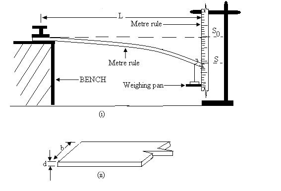Fig. 28 .

(a) Clamp the metre-rule firmly with a distance L of about 90 cm. Overhanging from the bench. The free end is such that it acts as a pointer along the metre-rule clamped in the vertical position. Note the scale reading, S₀ on the vertical metre-rule when the horizontal metre-rule is not loaded.

(b) Fasten the weighing pan at the free end of the horizontal metre- rule with a piece of strong thread.

Add on to the weighing pan a mass, m of 20 g and record the scale reading S on the vertical metre- rule.

Calculate the depression, D = S - S_o, corresponding to the added mass.

Keeping the length L constant, add a series of masses from say 20 g to 150 g in steps of 10 g or 20 g.

With each added mass, record S and calculate D. (see Fig. 11 (i))

(c) Use vernier calipers to measure the breadth, b and thickness, d of the horizontal metre-rule. (see Fig. 11 (ii)).

(d) Plot a graph of depression, D against the added masses,m.

From your graph, determine:

(i) The slope.

(ii) Calculate the Young’s modulus, Y of the material of the metre-rule by using the formula:

Where g = 9.8 ms^-2

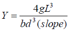
Experiment No. pM – 12

You are to find Young’s modulus of elasticity for wood by measuring the depression of a loaded half metre-rule.

Proceed as follows:-

Clamp the two half metre-rules firmly between the wooden blocks with a length L = 450 mm projecting as shown in Fig. 12

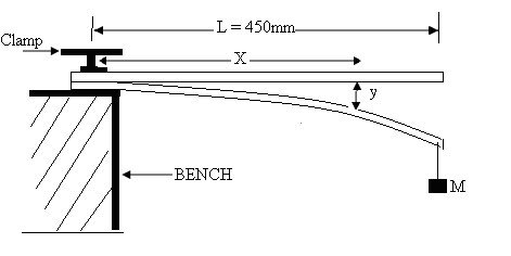
Fig. 29 .

Hang the mass, M over the end of the lower rule and measure the depression, y for different distances, x from the support.

Dismantle the apparatus and measure the width, a and the thickness, b of the halfmetre rule which had been loaded.

(i) Plot a graph of y against x.

(ii) Find the value,

when x = 300mm

(iii) Calculate a value for the Young modulus, E of the wood, given that:

Where: g = 9.8 ms^-2

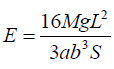
Experiment No. pM-13

The aim of this experiment is to determine the Young’s Modulus, E of elasticity of a cantilever.

Proceed as follows:-

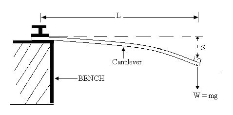
Fig. 30 .

Clamp the cantilever beam on a bench using a G-clamp as shown. Load the beam using the 200 g mass and fasten it rigidly at distance, L = 90 cm from the G-clamp.

Use the cello tape or any other means available for this purpose.

The load is affixed to the cantilever such as to cause but a small depression, S when the beam is at rest. Depress the load slightly so that it starts to vibrate.

Record the time for 20 complete oscillations and hence the period, T for one complete oscillation.

Repeat the above procedure for at least five more values of L, each time decreasing by 5 cm, changing the position of the 200 g mass; the clamped end should not be disturbed.

For each value of L determine the time, and the period, T.

Neatly tabulate your results.

If the period of oscillation, T is related to the length, L by:

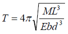
Where M is the load, b and d are the width and thickness respectively; then plot a graph of T² against L³.

Use your graph to calculate:

(i) The slope of the resulting graph, and hence (ii) The Young’s Modulus, E.

Experiment No. pM – 14

Use the experimental procedure outlined below to determine the viscosity,  of liquid L.

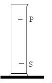
Fig. 31 .

You are provided with a measuring cylinder, glycerine, stop-watch, small steel ball bearings of varying diameters, micrometer screw-gauge, metre rule, hydrometer, and thermometer (0 – 100^oC).

Proceed as follows:

Measure the diameter of each steel ball bearing and also measure the density and temperature of glycerine.

Fix a mark, P with a sticky label well below the top of the liquid and fix a second mark, Q near the bottom of the cylinder.

Measure the distance, S between P and Q.

Fill the measuring cylinder with glycerine, and then drop in the largest steel ball bearing.

Record the time, t of fall of the steel ball bearing between the marks P and Q.

Do the same with the other steel ball bearings and tabulate your results as indicated below:

Diameter of	r2	S	t	v
balls (cm)	(cm2)	(cm)	(s)	(cms-1)

Where: r is the radius of the steel balls and v is velocity.

(a) Plot a graph of r² against v and find its slope.

(b) Find the viscosity,  of the liquid, given that:-

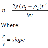
Density of steel, ρ₁ = 7.7 x 10³ kgm^-3 Density of glycerine, ρ₂ = 1.26 x 10³ kgm^-3 g = 9.8ms^-2

(c) What is the temperature of glycerine?

Experiment No. pM – 15

The aim of this experiment is to investigate the flow of water in a constricted vertical tube.

Proceed as follows:-

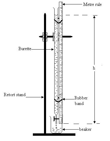
Fig. 32 .

(a) (i) Fix the burette on the retort stand so that it maintains an upright vertical position.

(ii) Fix the metre-rule beside the burette using rubber bands so that the zero end of the rule is on the same level as the ejecting end 0 of the burette.

(iii) Fill the burette with water to within 1.0 cm of the top.

(iv) Using the burette tap or clip adjust the water level L to a readable mark to enable the water head (height) h be recorded easily.

Record the initial value of water head h₀.

(v) Allow the water to run out of the burette and simultaneously start the stop-watch.

(vi) Record the water head h₁ at 15 seconds intervals in a tabular form (shown below) to obtain at least 10 readings of height h₁ and time t.

(vii) Repeat the experiment making sure that the same initial level L is maintained when the timing starts.

Record the water head h₂ against time t.

(viii) Obtain a column of average values of water head:

Time, t (s)	h1 (cm)	h2 (cm)	Water head (cm)

(b) (i) Plot a graph of water head, h(cm) as ordinates against Time, t (s) as abscissae.

(ii) On the graph locate points P₀, P₁ and P₂ corresponding to ordinates

Extract corresponding values of time T₀, T₁ and T₂.

(iii) Draw tangents to the curve at:

(iv) Determine the values of slope S₀, S₁ and S₂ corresponding to the three tangents drawn in (b) (iii) above.

These values represent the rate of flow decay dh/dt

(c) (i) dh/dt

Plot a graph of values of dh/dt against h.

(ii) Determine the gradient G of this graph.

(iii) Deduce the physical meaning of k = - G.

(iv) Write the relationship existing between dh/dt, h and k.

(v) What physical process does the curve in the first graph define?

(vi) What law governs the flow of water in a constricted vertical tube?

(vii) Suggest one other physical process which obeys the law stated in (c ) (vi) above.

(d) (viii) State any two sources of errors in this experiment.

Experiment No. pM – 16

You are required to determine the surface tensions _a of liquid A and _b of liquid B.

Proceed as follows:

Set up the apparatus shown in Fig. 16.

With the clip closed, fill the funnel with the liquid A.

Adjust the gripping of the clip so that the rate of issuing of the drops at the lower open end is between 20 and 30 drops per minute. Initially, when making the adjustments the drops may be collected in the measuring cylinder.

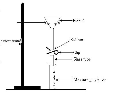
Fig. 33 .

Starting with a convenient reading V₀ of the volume of liquid already collected in the measuring cylinder, observe the new volume V of the liquid in the measuring cylinder when a known number n of drops has been collected.

Without losing the sequence of count of n, observe series of pairs of V and n.

Tabulate your observations.

Plot a graph of V-Vo (vertical axis) against n.

Assuming that the drops are all equal, determine from the resulting graph the diameter, d and the mass, m_a of one drop.

Hence using Lord Rayleigh’s formula:

Where: g = 9.8 ms^-2, the acceleration due to gravity.

Calculate γ_a.

You may assume that the density of the liquid A is 1.0cm^-3.

Now empty the entire apparatus and refill it with the liquid B. Adjust the rate of flow as before.

Collect 10 drops of the liquid B into the small beaker and contents so as to obtain the mass of 10 drops of the liquid.

From your observations determine the mass m_b of one drop.

Calculate the surface tension, γ_b of the liquid B given that:

Where: g and d have the same values as above.

Assume that the density of the liquid B is 0.85 gcm^-3