Chapter 02 : National income
| Introduction At the micro level, income is one of the determinants of welfare of an individual. However; at the macro level national income is used to determine the economic performance of a nation. In this chapter, you will learn about the concept of national income, measuring the national income, per capita income, determinants of the size of national income, and determination of national income equilibrium. The competencies developed will enable you to interpret national income data and use them to explain changes in economic performance and living standards. |
| Think Existence of countries without national income. |
Activity 2.1
Search from different sources, including online for different key terms related to national income.
The concept of national income
National income is the total monetary value of all final goods and services produced by factors of production in a certain country over a period of time, usually one year. It aggregates all incomes which arise from current production of goods and services in the economy. National income is always measured in monetary terms. In the modern economy, there are various concepts used to measure the market values of goods and services produced in the economy.
Key terms related to national income
Various terms are used to describe the national income. These terms differ in items that are included or excluded in the calculation of national income. The terms are described as follows:
National expenditure: Refers to total spending on domestically produced final goods and services by all households, government, investors, and the rest of the world during a specific period (usually a year) National output: Refers to total value of output (goods and services) produced in the country during a particular year. In value, national output is exactly equal to national expenditure.
Gross Domestic Product (GDP): Refers to the total market value of all final goods and services produced within a country in a certain period, usually one year. GDP measures two things at a time. On one hand, GDP measures the total income earned by factors of production, and on the other hand it measures total expenditure on goods and services in an economy. One thing to note is that, GDP should be measured using the market value of the final goods and services produced by citizens and non-citizen within a particular country. The GDP identity can be written as the sum of consumption expenditure on final goods (C), investment expenditure on intermediate goods (I), government expenditure on goods and services (G), and net export of goods and services (X – M). Where X represents exports of goods and services and M represents imports of goods and services.
- GDP = C + I + G + (X – M) . . . . . . . . . . .. (2.1)
Economists often use GDP to measure economic prosperity of the country. A higher GDP level signifies a higher level of well-being of the people.
Depreciation: Refers to loss of value of the economy’s capital assets such as stock of equipment and structures due to wear and tear. In national income accounting, the depreciation of capital assets is also known as consumption of fixed capital/assets.
Gross National Product (GNP): Refers to the market value of all final goods and services produced in a given period usually one year by the citizens of a particular country regardless of their location. It includes income of all factors of production of the citizens living within and outside the country.
Gross National Product = Gross Domestic Product + Net factor income from abroad (NFIA)
- GNP = C + I + G + (X–M) + NFIA . . . . . . . . . . (2.2)
Net factor income from abroad: Refers to the difference between the country’s earnings from abroad and its payments to the rest of the world.
Net Domestic Product (NDP): Refers to the market value of all final goods and services produced within the country by both citizens and non-citizens minus losses from depreciation during a given period, usually one year.
- Net Domestic Product = Gross Domestic Product – Depreciation
NDP = Gross Domestic Product – Depreciation . . . . . . (2.3)
Net National Product (NNP): Refers to the market value of all final goods and services produced by the citizens regardless of their location in a given period minus losses from depreciation. The national income is identical to net national product but sometimes the difference occurs because of measurement error (statistical discrepancy).
- Net National Product (NNP) = Gross National Product – Depreciation . . ..(2.4)
Personal Income (PI): Refers to the income received by the individuals or households from all sources before the deduction of all direct taxes. Personal income is not equal to national income because personal income includes the transfer payments, while national income does not. Personal income is derived from national income by deducting undistributed corporate profits and taxes, and employee’s contributions to social security schemes such as pension funds.
Personal Income = National Income – Social Security Contributions – Corporate Taxes – Undistributed Corporate Profits + Transfer Payments . . ..(2.5)
Disposable income (DI): Refers to the income of the individuals after deduction of all direct taxes. It is the income ready for consumption and saving.
Disposable Income = Personal Income – Personal Taxes . . ..(2.6)
Disposable income can be used either for consumption or saving. The amount that is not consumed is saved. If we denote the disposable income by DI, consumption by C and saving by S, the disposable income can be expressed as:
- DI = C + S . . . . . . . . . . . . . . . . . . ..(2.7)
The amount saved is normally used to generate some capital which is used to earn more income. This is known as investment (I). It is the amount saved which is turned into investment. Therefore, from this logic, the disposable income can also be expressed as:
- DI = C + I . . . . . . . . . . . . . . . . . . ..(2.8)
From equations (2.7) and (2.8), it is logical to say that saving is equal to investment if the economy is in equilibrium. This means that all saved amounts are converted to investment, as expressed in equation (2.9).
C + S = C + I
C – C + S = I
- S = I . . . . . . . . . . . . . . . . . . ..(2.9)
Nominal GDP: Refers to the measure of the GDP for a particular period using the actual market prices in that period usually a year. This gives us the nominal GDP or GDP at current market prices. However, the interest is to determine what happens to the real GDP.
Real GDP: Refers to the market value of all final goods and services produced in a certain period of time, usually one year, and is measured at constant prices of a chosen year (base year price). Unlike the nominal GDP, real GDP is calculated by taking the volume or quantity of production after removing the influence of changing prices or inflation.
Per capita income: Refers to the average income of the people in the country in a particular year. It is sometimes known as income per person.
Measuring the national income
To understand how national income is measured, let’s begin with a simple model called circular flow model of income in the economy. The simple circular flow model of income is a hypothetical concept in which it is assumed that there are only two sectors: firms and households. It diagrammatically represents the flow of goods and services as well as expenditures across firms and households via product and factor markets without government interventions and trade with other countries. This model is presented in Figure 2.1.
|
Figure 2.1:The circular-flow model of income |
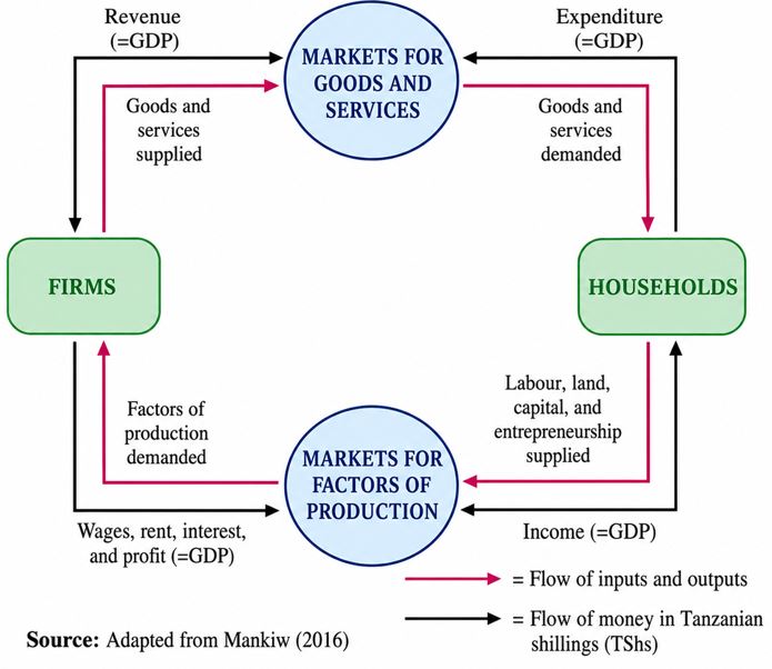
In Figure 2.1, firms hire factors of production: labour, land, capital, and entrepreneurship from the households. Households in turn receive income in the form of rent, wages, interest and profits. The firms use these factors of production to produce goods and services; and households buy the goods and services produced by firms. Firms earn revenue from the households. Thus, the total income received by households must be equal to the revenue earned by firms from expenditure of households. The inner arrows in the diagram shows the flow of factor inputs and goods and services between businesses and households; while the outer arrows show the flow of money payments made by business to buy factor inputs and households to buy goods and services produced by business. Without loss of generality, note that, the outer arrows can be expressed in terms of income received by selling factor inputs; wage for labour, interest for capital, rent for land and profit for entrepreneurship.
Figure 2.1 suggests three ways of measuring national income. Final outputs at market price, total expenditure on goods and services at market price, and income received by households for selling factor inputs. Therefore, derived from these facts, there are three methods of measuring national income: output, income, and expenditure methods.
Output method or product method: In this method, the GDP is obtained by adding up the value of output produced at each stage of production. The output method of computing GDP is sometimes known as the value added method because it includes only the values of intermediate goods (net value of all output) produced in a given year to avoid double counting. The method does not add up the values of all output produced at each stage of production rather it add up only the added value at each stage of production. Value added is the difference between the market value of the output of the business and the cost of inputs purchased from other businesses.
For example, a farmer sold a kilogram of rice to a miller for TShs 2,000. The miller turns the rice into flour and then, sells the flour to the food restaurant for TShs 6,000. The food restaurant uses the flour to make vitumbua and sells them to students for TShs 12,000. Assuming that only one kg of rice is produced in this economy the computation of GDP by using output method is illustrated in Table 2.1.
Table 2.1: The output method for measuring GDP (in TShs.)
| Sector | The value of output | The value added |
| Farmer | 2,000 | 2,000 |
| Miller | 6,000 | 4,000 |
| Food restaurant | 12,000 | 6,000 |
| GDP | 12,000 | |
Table 2.1 illustrates that, the value added of each sector is computed and then, these values are aggregated to obtain the GDP. Another example of computing GDP using National Bureau of Statistics (NBS) data of the year 2019 is illustrated in Table 2.2 by the output method. It is important to note that, GDP measured this way value the goods and services before they enter into the market. Hence, it excludes taxes on the products. To obtain GDP at market prices, taxes on product has to be added.
Income method: In this method, the GDP is computed by adding up the distribution side of income. The GDP is computed by adding up all income earned by factors of production during a period of one year. Therefore, the national income is computed by summing up rents from land, interests from capital, profits from entrepreneurs, and wages and salaries from employees. It is further presented mathematically as,
- National Income (Y) = Interest (I) + Rent (R) + Wage (W) + Profit (P) . .(2.10)
Although the National Bureau of Statistics (NBS) does not publish data on national income computation using income method, the same can be computed from data obtained in the computation of national disposable income and its appropriation. NBS uses compensation of employees, which is total remuneration payable by enterprises to employees, and operating surplus, which is surplus accruing from production (profit, rent and interest) before deduction of tax. The sum of these provides net domestic income at factor cost (or basic prices). By adding consumption of fixed capital and taxes of products, we obtain GDP at market prices using the income method as shown in Table 2.3.
- Table 2.2: National income computation using the output method
| Economic activity | Value added (million in TShs.) |
| Agriculture, forestry and fishing | |
| Crops | 20,632,396 |
| Livestock | 10,344,727 |
| Fishing | 2,379,172 |
| Forestry | 3,738,360 |
| Agriculture support services | 42,136 |
| 37,136,791 | |
| Industry and construction | |
| Mining and quarrying | 7,219,118 |
| Manufacturing | 11,872,086 |
| Electricity supply | 374,002 |
| Water supply; sewerage, waste management | 628,187 |
| Construction | 19,944,486 |
| 40,037,879 | |
| Services | |
| Wholesale and retail trade; repairs | 12,264,410 |
| Transport and storage | 9,621,651 |
| Accommodation and food services | 1,770,670 |
| Information and communication | 2,052,242 |
| Financial and insurance activities | 4,927,613 |
| Real estate | 3,831,113 |
| Professional, scientific and technical activities | 903,234 |
| Administrative and support service activities | 3,640,720 |
| Public administration and defence | 5,357,235 |
| Education | 3,322,488 |
| Human health and social work activities | 1,932,659 |
| Arts, entertainment, and recreation | 427,887 |
| Other service activities | 1,140,424 |
| Activities of households as employers | 241,246 |
| 51,433,592 | |
| All economic activities at basic prices | 128,608,262 |
| Add: Taxes on products | 11,285,542 |
| GDP at market prices | 139,893,804 |
Source: National Bureau of Statistics (NBS), 2022
Table 2.3: National income computation using income method
| Types of income | Income (million in TShs) |
| Compensation of employees | 44,056,615 |
| Operating surplus | 61,334,955 |
| Net domestic income at factor cost (basic prices) | 105,391,570 |
| Add: Taxes on products | 11,285,542 |
| Net Domestic at market prices | 116,677,112 |
| Add Consumption of capital | 23,216,692 |
| GDP at market prices | 139,893,804 |
Source: NBS (2022)
Expenditure method: In this method, the GDP is computed by summing up all the final expenditures on goods and services produced in one year. The GDP is obtained by adding up consumption expenditure made by households, investment expenditure by firms, government spending and net exports. The expenditure method of measuring GDP can be expressed using the GDP identity, as the sum of personal consumption expenditure on the final goods (C), gross domestic investment expenditure (I) on intermediate goods (I), government expenditure on goods and services (G), and the net export of goods and services (X−M). Where X denotes export of goods and services and M represents import of goods and services. Recall equation (2.1) which is, GDP = C + I + G + (X − M)
The example of GDP computation using NBS data of the year 2019 is illustrated in Table 2.4 by the expenditure method.
Table 2.4: National income computation using expenditure method
| Type of expenditure | Value (million in TShs) |
| Final consumption | |
| Government final consumption | 10,867,505 |
| Household final consumption | 81,601,115 |
| Non-profit institutions serving households | 311,653 |
| 92,780,273 | |
| Gross capital formation | |
| Gross fixed capital formation | 59,529,980 |
| Changes in valuables | 273,337 |
| Changes in inventories | -5,328,628 |
| 55,474,689 | |
| Exports of goods and services (X) | |
| Export of goods | 12,597,462 |
| Export of services | 9,796,547 |
| 22,394,009 | |
| Imports of goods and services (M) | |
| Import of goods | 19,681,869 |
| Import of services | 4,031,891 |
| 23,713,760 | |
| Exports – imports (X – M) | -1,319,751 |
| Errors and omissions | -7,041,408 |
| GDP at current market prices | 139,893,803 |
Source: NBS (2022)
It is important to note that in theory, all the three methods of computing national income give the same figure of national income. Referring to Tables 2.2, 2.3 and 2.4 respectively, the national income computed from output equals the income and expenditure methods. This can simply be expressed as,
- Value of National Output = Value of National Income = Value of National Expenditure
But practically, data are not perfect; therefore, the national income figures computed using different approaches may slightly differ. The slight difference in figures is known as statistical discrepancy.
Furthermore, GDP can be expressed either using current (prevailing) market price of goods and services or the costs used to produce goods and services. Therefore, there is GDP at factor costs and GDP at market price. The GDP at market price is obtained by taking GDP at factor cost plus the indirect taxes minus subsidies.
- GDP at market price = GDP at factor cost + indirect taxes – subsidies . . .(2.11)
GDP at factor cost is obtained by taking GDP at market price plus subsidies minus indirect taxes.
- GDP at factor cost = GDP at market price + subsidies – indirect taxes . . .(2.12)
Activity 2.2
1. Visit a school library, government websites and read economic survey reports of Tanzania. Collect data on the GDP of Tanzania for the past five years, then:
(a) Describe a trend of GDP of Tanzania; and
(b) Is there any difference between your findings and those of your fellow students? If the answer is yes, explain.
2. Collect and record previous year economic data from Tanzania of all expenditure items, output of all sectors, and income received by all factors of production, then:
(a) Compute the GDP and Net National Income (NNI) using the three approaches;
(b) Are the GDP figures computed in (a) the same or different? Explain the reasons.
Uses of national income statistics
National income statistics are figures produced/calculated to assess the economic performance of a particular country. These statistics include but not limited to GDP, GNP, and per capita income. The uses of national income statistics are crucial in the economy. The following are some of the important uses of national income statistics:
It helps to determine the distribution of income among the factors of production:
The statistics show how national income is distributed among different actors in the economy. For example: wage earners, rent earners, interest earners and profit earners.
It helps to compare the level of standard of living across countries: The figures of real national income and the per capita income are used to compare the standard of living in different countries. Therefore, the higher the per capita income, the higher the standard of living in a country and vice versa.
It is used to formulate national economic plans and policies: By using the national income statistics, it is possible to know the contribution of each sector to the national economy. The statistics are relevant for the government to decide on the regulation and stimulation of its sectors. Firms and the government can plan to use the available resources to stimulate or regulate agriculture, industry, infrastructure and social services for economic development.
It helps to show the overall economic performance: The national income seeks to measure the value of production in a year. The statistics will show whether the economy is growing overtime or not. Therefore, the statistics helps to compare the level of economic performance over time.
It helps to show the contribution of each sector in the economy: The national income statistics help to know the sectoral contribution to the overall economy. For example, in Tanzania agriculture sector is the most contributing sector to the economy's GDP and employment. The United Republic of Tanzania country's survey report of 2020 reveals that the agricultural sector contributed about 26.9 percent of the economy's GDP.
It helps to determine the growth rate of an economy: The data on consumption, saving and investment are important in determining the economic growth of the country. However, consumption and investment are the components of the aggregate demand which depend on the level of income and employment in a country. Therefore, an increase in these components will indicate whether the economy is growing or not.
Problems in measuring national income
The process of measuring national income is not straight forward, since there are various challenges that arise in the process of computation. The following are the problems experienced in measuring the national income:
Problem of double counting: The value of intermediate goods such as raw materials or inputs should not be part of GDP because their cost is already included in the price of final goods and services. Therefore, including it will lead to double counting. Thus, all goods and services produced by one firm for another should not be included in the national income computations. This is because the value of the mentioned goods and services have already been included in the price of final product. For instance, services like banking, transportation, and insurance should be excluded because they are included elsewhere.
Non-inclusion of non-market goods and services: Gross Domestic Product (GDP) measures the market value of all final goods and services but not goods and services which no market value. Examples of goods with no market values are vegetables and fruits that are consumed from gardens at homes. These goods are not included in the GDP calculations. Similarly, traditionally housewives do most of house works for the family. These are not included in the GDP because there is no established market price for them. Housewives offer the same services like those offered by maid servants employed in the hotels; but only the activities of maid servants are included in the GDP. A balanced approach would include services of the housewives in calculating GDP because they are economic activities performed in the economy.
Inadequate statistical data: Most of economic activities conducted in the economy are not recorded properly. One of the reasons is that most individuals, firms, and government institutions do not keep records properly. The other reason owes to economic informality. Thus, most of the national income figures are computed based on estimates from samples which may result into either underestimation or overestimation of GDP figures.
Estimation of depreciation allowance: In order to come up with the Net National Product (NNP), depreciation is deducted from GNP. But the problem arises in estimating the current depreciation value of capital goods that has lasted for a long period of time such as thirty years or more. Firms calculate the depreciation value on the original cost of the capital goods to determine their expected life. However, this does not solve the problem because the prices of capital goods change almost every year.
Price changes: National income is computed by using the market value of goods and services at current market prices. But prices are not stable, they fluctuate from time to time. When the price level rises, the national income also rises, though the national production might have fallen. On the other hand, when price level falls, national income also falls, though the national production might have increased. As a result, price changes do not adequately measure national income. That is the reason economists prefer to compute real national income at constant prices by using the price index known as GDP deflator.
Income from illegal activities: Income earned from illegal activities like corruption, prostitution and smuggling are not included in the national income. Such activities have undesirable effects and are not considered productive from the point of view of the society. This, however, may not be the case for the other countries where such activities are legal.
Treatment of government services: Most of the government services that are provided for free to the population must be included in the computation of GDP. However, it is difficult to find the value of these services since they are not sold via market channels.
Externalities: Effect of the action of one agent that affect another economic agent who is not part of that action is not captured when measuring national income. For example, the effect of a mining company polluting water that is used by villagers living adjacent to the mine is not captured.
Per capita income
Refers to its definition, the per capita income is computed by dividing the Gross National Income (GNI) by the total population of a particular country as shown in the formula (2.13). Per capita income is used to determine average income per person in a given country. It is an important variable for the evaluation of the standard of living of a population.
Per capita income = Gross National Income/Total population . . . . (2.13)
where:
- National income = GNP or GNI (depending on the measure used)
- Total population = The number of people in the country
Interpretation:
(a) A high per capita income means on average people in the country earn more, suggesting better living standards (though it does not show income distribution).
(b) A low per capita income suggests lower average earnings and possibly lower living standards.
Weaknesses of using income per capita to compare standard of living
High per capita income implies high standard of living because per capita income is usually used to compare living standard across countries overtime. A country with a high per capita income enjoys high living standard while a country with a low per capita income does not. However, per capita income is not a perfect measure of standard of living and, therefore, provides a challenge of using it to compare the standard of living across countries. There are several weaknesses of using per capita income to compare living standards among the nations. These weaknesses include the following:
Differences in taste and preference: People from different countries have different tastes and preferences. For example, due to geographical differences a person living in Europe has to spend more on in-house heating during winter than does a Tanzanian due to the variations in climatic conditions. Obviously, neither the European nor the Tanzanian is better off in this aspect. However, when using the per capita income figures to compare their welfare, the figures may indicate that a European is better off than a Tanzanian.
Currency variations: The per capita income figures are expressed in different currencies. They have to be converted into a common currency in order to make proper comparison. Using the exchange rate for this purpose, however, is not conclusive. This is because the rate may not accurately reflect the internal purchasing power of a currency.
Countries differ in spending: The proportion of income spent by different countries on defence and non-welfare improving activities vary. Countries which spend less on non-welfare improving activities can enjoy consuming goods and improve standard of living, but per capita income does not indicate these differences.
Variations in length of the working hours: Countries vary with regard to the length of the average working hours and the proportion of women who work. It may happen that, the high per capita income in one country is a result of working for long hours while sacrificing leisure. However, per capita income measure does not show this fact.
Per capita income does not show income distribution: There is another possibility of the per capita income not being able to increase economic welfare when real per capita income declines. A small percentage of the population may be controlling a large share of GDP. For example, if the increased income goes only to the few rich people, the per capita income will not increase economic welfare of the majority of the population.
Per capita income fails to measure adequately changes in the value of output due to changes in the price level: Price index used to measure price changes are simply approximations. Thus, they cannot adequately measure economic performance.
The increase in per capita income may not raise the real standard of living of all people:It is possible that while per capita real income is increasing, per capita consumption might be falling. People might be using the increased income to increase their saving.
It fails to take into account the increase in standard of living associated with social factors: The improvement in living standards comes from education, nutrition, health and housing, cannot be measured by the increase in per capita income.
It does not consider issues of externality: The outcome of per capita income is calculated without considering the issue of externality.
Exercise
1. Using a two-sector circular flow model of income, explain how economic agents interact in the factor markets and product markets.
2. The production of goods and services inside or outside the domestic economy by citizens and non-citizens makes the concepts of national income and GDP to be defined differently. Justify this statement.
3. Explain the challenges of using per capita income as a measure for comparing standards of living across countries.
4. With examples, explain how the national income statistics help the government and citizens in making investment decisions and understanding living standards.
www.learninghubtz.co.tz
Exercise
1. Using a two-sector circular flow model of income, explain how economic agents interact in the factor markets and product markets.
2. The production of goods and services inside or outside the domestic economy by citizens and non-citizens makes the concepts of national income and GDP to be defined differently. Justify this statement.
3. Explain the challenges of using per capita income as a measure for comparing standards of living across countries.
4. With examples, explain how the national income statistics help the government and citizens in making investment decisions and understanding living standards.
Determinants of the size of national income
There are number of factors that determine the level of national income of a given country. Some of these factors are explained as follows:
The stock of natural resources: Natural resources such as minerals, fertile land, water resources, and forest resources are relevant raw materials for the production of goods and services. The country that is rich in natural resources can achieve some level of production from the use of her natural resources. Consequently, the high level of production will increase aggregate output which further translates to the country’s national income. On the other hand, a country which is poor in natural resources will fail to increase production and, therefore, the size of national income will be low.
The size of skilled labour force:Labour force is an input used in the production process. A large stock of skilled labour force will be more efficient/productive in the course of producing goods and services. The raised productivity may lead to high national income. On the other hand, a small stock of unskilled labour is associated with small size of national income.
Size of capital stock: Capital goods help to increase productivity of other factors of production. A country with a large stock of capital is able to raise its production levels leading to high size of national income. On the other hand, the presence of insufficient stock of capital leads to a small size of national income.
Entrepreneurial skills: Experienced and skilled entrepreneurs lead to efficient organisation of other factors of production leading to greater productivity and, hence, raise the size of national income. On the other hand, a country with unexperienced and unskilled entrepreneurs will experience a small size of national income.
The level of technological advancement: High technological progress may lead to high output from the use of fixed resources. The same output can be obtained by the use of a small quantity of resources due to technological advancement. Low level of technology leads to small national income levels.
Determination of national income equilibrium
The equilibrium level of national income is determined by the interaction between aggregate supply (AS) and aggregate demand (AD). In a simplified model this level of national output and income settles at a point where it neither expand nor contracts as shown in Figure 2.2
|
Figure 2.2: Equilibrium national income (AS & AD) |
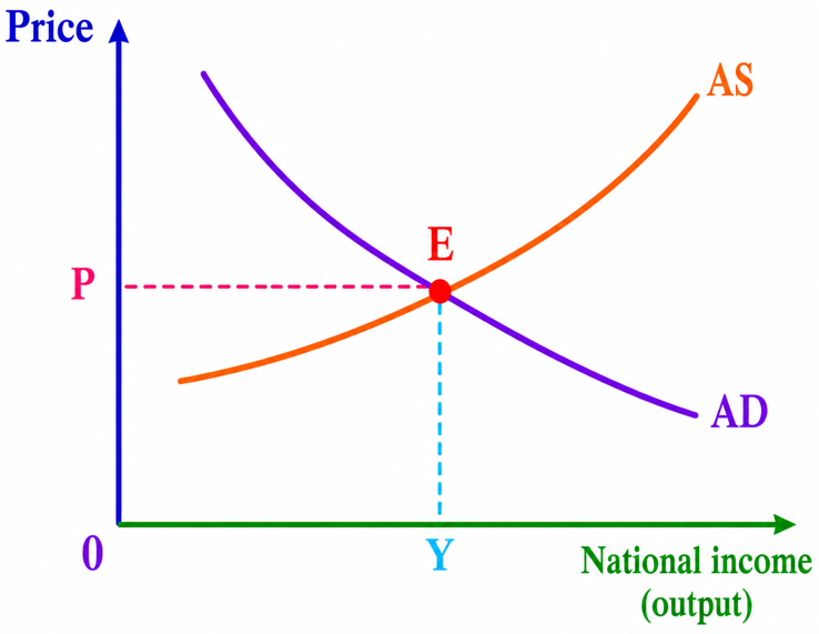
Aggregate supply of goods and services in a country depends on the productive capacity of the economy. On the other hand, aggregate demand depends on the willingness and ability of the people and firm to spend on consumption of goods (C) and on investment of goods (I). Therefore, aggregate demand (AD) can be expressed as: AD = C + I …………………… .(2.14)
According to Keynes, the national income: Y = C + I = Aggregate Demand as shown in Figure 2.3.
|
Figure 2.3: Equilibrium national income (AE & AD) |
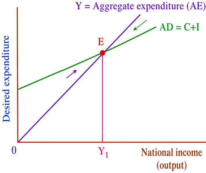
But income has another side, which is spending side. From this point of view, income is spent on consumption and saving. Therefore, income is expressed as:
AS = C + S . . . . . . . . . . . . . . . . . . . . ..(2.15)
According to Keynes, the national income: Y = C + S = Aggregate Supply.
The equilibrium level of national income is determined by bringing together equations (2.14) and (2.15). Thus, the equilibrium level of national income is attained when total injections equal to leakages. In a closed economy in the absence of government sector, the autonomous investment is the only injection and saving is the only leakage. Thus;
Y = Aggregate Demand = C + I
Y = Aggregate Supply = C + S
Given that, Aggregate demand = Aggregate supply, then,
C + I = C + S
C - C + I = S
I = S = equilibrium level of income . . . . . . . . . . . . ..(2.16)
Saving = Investment
Therefore, equilibrium national income determination of leakages-injections approach can be termed as saving-investment approach. At equilibrium, the savings (leakages) must be equal to investment (injections).
In Figure 2.4, the national income is at equilibrium when saving (leakages) is equal to investment (injections) at point E. If savings (leakages) exceed investment (injections), then total expenditure will decline, and the result is to decrease output. On the other hand, if investments exceed savings, then total expenditure will increase, and the result is an increase in output. Only when investments and savings are equal at point E, output will remain the same at Y₁.
|
Figure 2.4: Equilibrium level of national income |
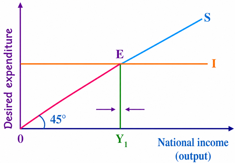
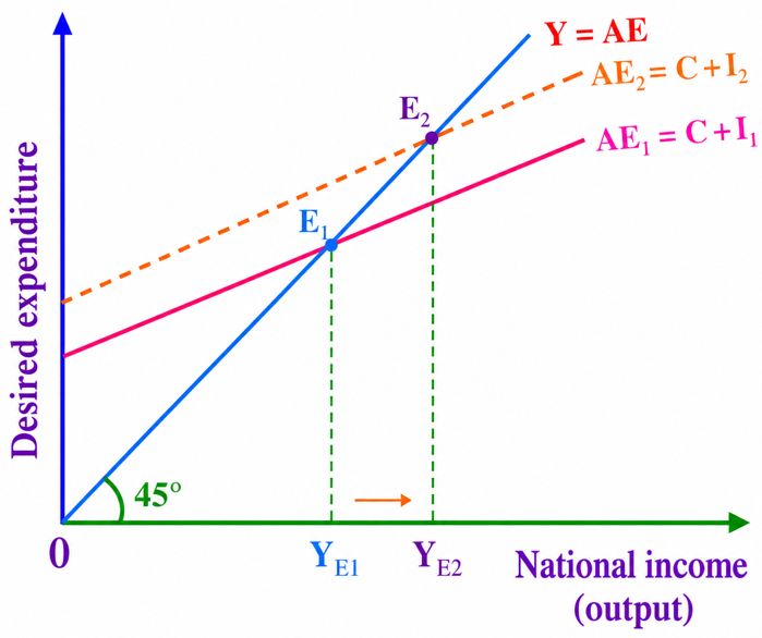
In Figure 2.5, the shift in aggregate expenditure curve (AE) leads to changes in equilibrium national income. For example, suppose aggregate demand increases from AE₀ to AE₁ as a result of increase in investment expenditure, equilibrium level of national income increase from Y₁ to
|
Figure 2.5: National income determination by consumption and investment |
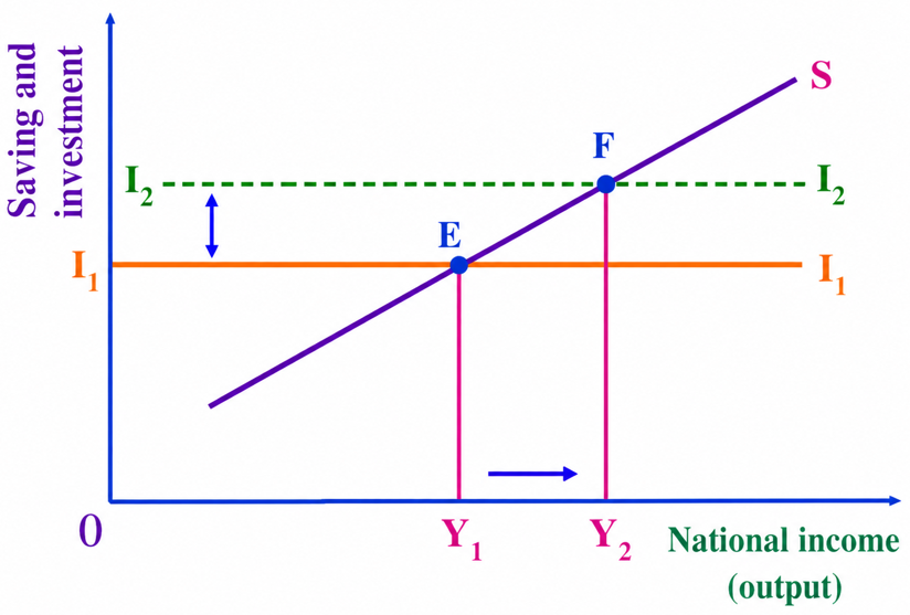
The changes in equilibrium national income can either be a result of an increase or shift in savings or investment curves. For example, a rise in investment expenditure will shift the investment demand curve upward from I₁ to I₂, the result is an increase in equilibrium level of national income from Y₁ to Y₂, as depicted in Figure 2.6.
|
Figure 2.6: Income determination by saving and investment |
Consumption function
A consumption function is the expression of relationship between consumption and disposable income. Consumption spending of the people is influenced by the following factors among others: the disposable income of the individual, past saving of the individual, and the rate of interest. The disposable income seems to be the strongest factor among all. Thus, the level of consumption depends on the level of income.
C = f(Y), function of income
The function f(Y) can take variety of forms but we can assume to take a linear form. As a result of this, the generalconsumption function in a linear form is usually expressed as:
C = a + bY . . . . . . . . . . . . . . . . . . ..(2.17)
Where: C represents the consumption level, “a” represents autonomous consumption, “b” represents marginal propensity to consume (MPC) which is the slope of the consumption function and “Y” is the disposable income.
However, there is a certain level of consumption known as autonomous consumption that does not depend on the level of income. It represents part of consumption spending from other sources than disposable income including past savings. It is also the vertical intercept of the consumption function.
Marginal propensity to consume (MPC)
Marginal propensity to consume is a parameter which shows the effect of an additional shilling of disposable income on consumption. Marginal propensity to consume is the proportion by which consumption spending changes resulting from a unit change in income. In other words, marginal propensity to consume is the ratio of change in consumption to change in income. For example, if your income increases by Tshs 40,000, 0.8 of this amount may be devoted for consumption and 0.2 for saving. This fraction of change in consumption over the change in income (which is 0.8 in the example) is what is referred to as the marginal propensity to consume. The MPCis computed using the formula in equation (2.18).
Marginal propensity to consume = Change in consumption
Change in income
MPC = ΔC/ΔY . . . . . . . . . . . . . . . . . . ..(2.18)
Where ΔC = change in consumption
ΔY = change in income
From the equation (2.17) of consumption function, C = a + bY
ΔC/ΔY = Δa/ΔY + bΔY/ΔY
ΔC/ΔY = 0 + b, where we make use of the fact that change in a constant number is equal to zero.
Therefore, MPC = ΔC/ΔY = b . . . . . . . . . . . . . . .(2.19)
Where 0 ≤ b ≤ 1
Average propensity to consume (APC)
Average propensity to consume refers to consumption per income. It shows the percentage of income that is spent on consumption. In other words, average propensity to consume is the ratio of consumption to income. The APC is computed using the formula in equation (2.20).
Average propensity to consume = Consumption/Income
APC = C/Y . . . . . . . . . . . . . . . . . . ..(2.20)
Determinants of the propensity to consume
Marginal propensity to consume is influenced by the following factors:
Income redistribution: Redistribution of income in favour of the poor tends to increase the propensity to consume. This is because the marginal propensity to consume of the low-income groups is high in comparison to that of the rich.
Increased wages: Increase in wage may affect MPC positively. If wages are increased, it will have a direct effect in shifting the consumption function upward.
Social security measures: Social security measures tend to increase the consumption function in the long run. The provision of unemployment relief, medical facilities, and old age pension, remove future uncertainty and the tendency to save is reduced, therefore, leading to an increase in consumption.
Credit facilities: Cheap and easy credit facilities help in shifting the consumption function upward. When loans are easily and cheaply available to the people, more durable consumer goods are purchased resulting to a rise in the propensity to consume.
Development of the means of transport and communication: Well-developed means of transport and communication tend to shift the consumption function upward. The movement of goods become easy, the size of the market expands and prices may fall due to the reduction of transport costs.
Saving function
Saving function expresses a relationship between the level of saving and disposable income. The level of saving depends on the level of disposable income. The saving function can be derived from aggregate supply as follows:
- Recall equation (2.15) which is, AS = Y = C + S
Where; Y is income level, C is consumption level and S is saving level. However, equation (2.17) represents the consumption function which is expressed as;
C = a + bY
Then, substitute equation (2.17) into equation (2.15) to have,
Y = a + bY + S
S = Y − a − bY
S = −a + (1 − b)Y . . . . . . . . . . . . . . . ..(2.21)
Therefore, equation (2.21) represents saving as a function of income.
Marginal propensity to save (MPS)
Marginal propensity to save is a fraction that shows an effect of additional shilling of disposable income on saving. In other words, marginal propensity to save is the ratio of a change in saving and a change in income.
Marginal propensity to save = Change in saving / Change in income
MPS = ΔS/ΔY . . . . . . . . . . . . . . . . . . ..(2.22)
From the saving function: S = −a + (1 − b)Y
Then, a change of S with respect to no change of Ycan be expressed as;
ΔS/ΔY = Δ(−a)/ΔY + (1 − b)ΔY/ΔY
MPS = ΔS/ΔY = 1 − b, where ‘b’ is a marginal propensity to consume.
Where 0 ≤ (1 − b) < 1.
The important point to note here is that, MPC and MPS sum up to one. This can be expressed as:MPC + MPS = 1
This fact is derived from the following:
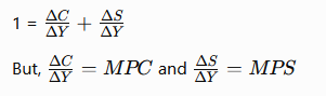
Y = C + S, since the change in income is associated with the change in consumption plus the change in saving, the following expression is valid;
ΔY = ΔC + ΔS
Divide by the change in income throughout the equation to obtain:
ΔY/ΔY = ΔC/ΔY + ΔS/ΔY
(b = 0), if the entire additional income is saved
(b = 1), if the entire additional income is consumed, indicating that income has no effects on saving.
Therefore, (MPC + MPS = 1) . . . . . . . . . . . . . . . ..(2.23)
Table 2.5 further elaborates on the computations of income, consumption, saving, average propensity to consume, average propensity to save, marginal propensity to consume, and marginal propensity to save.
Table 2.5: Income, consumption, saving and their propensities
| Income (Y) | Consumption (C) | Saving (S) | APC | APS | MPC | MPS |
| 1,000 | 950 | 50 | 0.950 | 0.050 | - | - |
| 1,100 | 1,040 | 60 | 0.945 | 0.054 | 0.9 | 0.1 |
| 1,200 | 1,125 | 75 | 0.938 | 0.062 | 0.85 | 0.15 |
| 1,300 | 1,205 | 95 | 0.927 | 0.073 | 0.80 | 0.20 |
| 1,400 | 1,280 | 120 | 0.914 | 0.086 | 0.75 | 0.25 |
Average propensity to save (APS)
Average propensity to save is saving per income. It is the percentage of income that is saved. In other words, average propensity to save is the ratio of saving to disposable income.
- Average propensity to save = Saving / Income
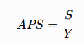 . . . . . . (2.24)
The important point to note here is that, (APC) and (APS) sum up to one, expressed as:
(APC + APS = 1)
This fact is derived from the following; (Y = C + S)
Divide by income (Y) throughout the equation to obtain:
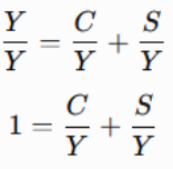

Therefore, (APC+APS=1) . . . . . . . . . . . . . . . ..(2.25)
Determinants of saving
Saving is determined by three major factors. These factors include the following:
Willingness to save: A portion of income can be saved only if a person has a desire to save. Willingness to save depends on the family affection, precaution, standard of living and social status. Thus, the higher the willingness to save the higher the savings.
Ability to save: Ability to save means the capacity to save. One cannot save without having the ability to save. The ability to save depends on factors like size of national income, natural resources, trade, industrial development, agricultural development, efficiency of labour, distribution of wealth and income.
Facilities and conducive saving environment: Saving depends also on the facilities and conducive saving environment such as peace and security, taxation policy, value of money, banking facilities, investment opportunities, and economic policy of the government.
Investment multiplier
Investment multiplier is a measure of the relationship between change in the equilibrium level of national income and the change in autonomous investment. Investment multiplier is the number of times by which change in investment has to be multiplied to get the resulting change in equilibrium national income. Investment multiplier is given by the following formula:

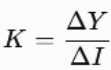
Where, (K) is investment multiplier, (Y) is income, and (I) is investment. The multiplier effect is the situation where initial change in the level of investment spending brings about more than a proportionate change in equilibrium national income. Figure 2.7 shows the investment multiplier in a saving and investment framework. The original equilibrium was at point E in which (Y_0) is an equilibrium national income. The increase in investment spending from (I_0) to (I_1), has the multiplier effect, since it increases the equilibrium national income from (Y_0) to (Y_1).
|
Figure 2.7: Multiplier in saving-investment |
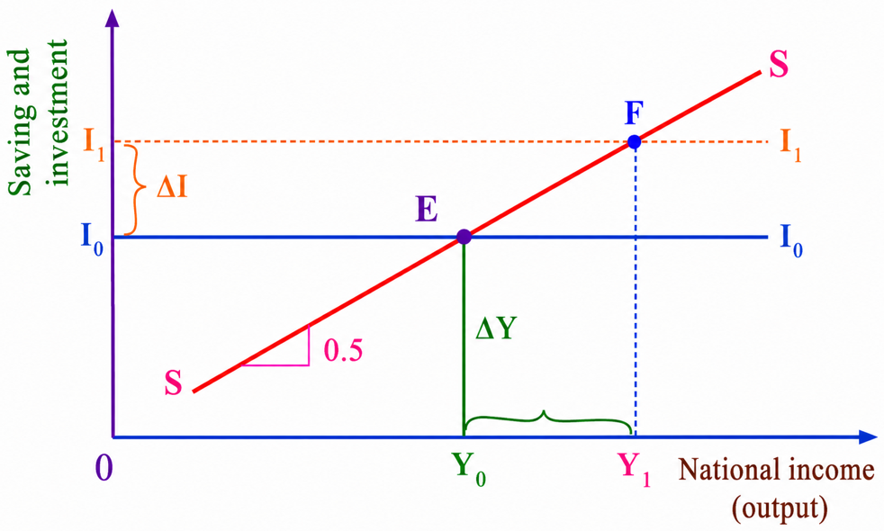
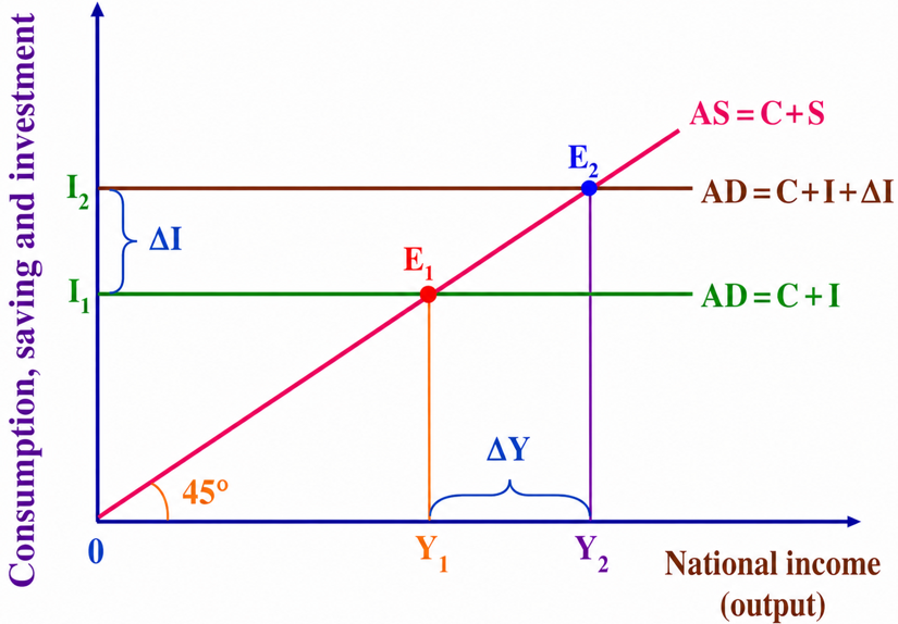
Figure 2.8 shows the multiplier effect using aggregate demand and aggregate supply framework. The initial equilibrium was at point (E_1), with equilibrium national income being at (Y_1), the increase in investment spending by (Delta I) has the multiplier effect because it increases the aggregate demand (AD) from (AD = C + I) to (AD = C + I + Delta I). The effect is increase in equilibrium national income from (Y_1) to (Y_2).
|
Figure 2.8: Multiplier in aggregate demand-aggregate supply |
Derivation of investment multiplier
In a closed economy and where there is no government sector, the aggregate demand is equal to consumption (C) plus investment (I); that is, (AD = Y = C + I), and the consumption function is given as (C = a + bY). From these equations, the investment multiplier can be derived as follows:
Given that,
Equation (2.14) is (Y = C + I) and equation (2.17) is (C = a + bY)
Substituting equation (2.17) into (2.14) to obtain equation (2.27):
(Y = a + bY + I) . . . . . . . . . . . . . . . . . . . .. (2.27)
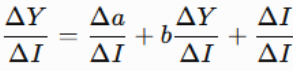
Then, find the first derivative or change of (Y) with respect to change of (I) by differentiating equation (2.27) to obtain equation (2.28).
 . . . . . .(2.8)

The derivative of any constant number equals to zero, plugging this expression in equation (2.28) and collecting the like terms we obtain the following:
 . . . . . . . . (2.29)
Since “b” is marginal propensity to consume (MPC), we can write
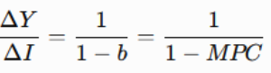
But, 1-MPC =MPS
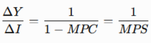
Therefore, The investment multiplier (K) is

Alternatively,
Given that;
C=a+bY . . . . . . . . . . . . . . . . . . . .. (2.30)
Y0=C+I0 . . . . . . . . . . . . . . . . . . . .. (2.31)
Substitute equation (2.30) into (2.31).
Y0(1-b) = a + I0
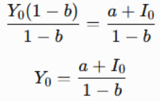 . . . . . . . . . . . .(2.32)
Where;
Y0 = Original income and
I0 = Original investment
Suppose income increases to (Y1) as a new national income level, then we write
Y1 = a + bY1 + I1
Collect like terms together
Y1 - bY1 =a + I1
Y1(1 - b) ==a + I1
Divide both sides by 1-b
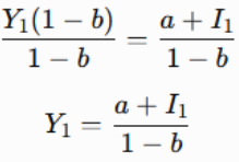 . . . . . . .(2.33)
The change in income is obtained by taking the equation (2.33) minus equation (2.32). That is,
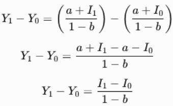
Assume no change in autonomous consumption
But, Y1 - Y0 =ΔY
I1 - I0 = ΔI
Therefore,

Divide both sides by ΔI


But also 1- MPC=MPS, therefore K= 1/MPS
Example 2.1
The marginal propensity to consume (MPC) of a certain economy is 0.75. The following procedures are followed to compute the investment multiplier.
Given the marginal propensity to consume is 0.75, we know that MPS = 1 – MPC. Therefore, the marginal propensity to save, MPS = 1 – 0.75 = 0.25.
Investment Multiplier (K) = 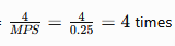
The multiplier of 4 means that the initial change in investment will be multiplied 4 times to obtain the final change in equilibrium national income.
Example 2.2
You are given the following consumption function and investment function; (C=200+0.80Y) and (I=50), respectively; where, (C) is consumption, (I) is investment and (Y) is disposable income.
Compute:
(a) The equilibrium level of income;
(b) The level of consumption at equilibrium; and
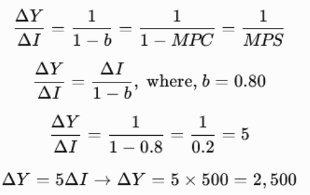
(c) The final change in national income given that change in investment is Tshs500.
Solution:
(a) The equilibrium level of income
Given that, (Y=C+I), where
C = 200 + 0.80Y and I = 50.
Since (Y = C + I), insert the consumption and investment equations into the income equation as follows:
(Y = 200 + 0.80Y + 50)
Collect the like terms on one side and solve for (Y).
(Y = 250 + 0.80Y) solving for (Y), therefore, (Y - 0.80Y = 250)
0.2Y = 250, divide both sides by 0.2
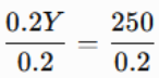
Therefore, Y=1,250
The equilibrium income is TShs 1,250
(b)
The level of consumption
Given that, C = 200 + 0.80Y and
Y = 1,250, substitute (Y) into consumption function.
C = 200 + 0.80 imes 1,250
= 200 + 1,000 = 1,200
Consumption is TShs 1,200.
(c)
Final change in national income
Given ΔI= Tshs 500 and C=200+0.8Y, then b=MPC=0.8
Investment Multiplier (K)=
Assumptions of the investment multiplier
The following are assumptions of the simple investment multiplier:
First, the investment multiplier assumes that the marginal propensity to consume is constant implying that, each round of new income generate a predictable constant fraction of new spending.
Second, investment multiplier assumes the economy operate below full employment level. Only with idle resources and increase in demand lead to a pure increase in investment, hence no inflation.
Third, the investment multiplier assumes that investment is autonomous meaning it is exogenous and not influenced by current income. It is independent shock that set multiplier process.
Fourth, the investment multiplier assumes that consumption is affected by current income; and the new level of investment is maintained steadily for the completion of the multiplier process.
Relationship between investment multiplier and marginal propensity to consume
The marginal propensity to consume (MPC) and the investment multiplier are directly related. That is, the larger the value of MPC, the larger the value of investment multiplier; and the lower the MPC, the smaller the investment multiplier. The value of MPC vary from 0 to 1 inclusive. Suppose the MPC is given by 0.99 which is very large, the investment multiplier will be  On the other hand, if the MPC is 0.10, which is small, the investment multiplier will be small
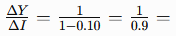 1.1 times.
Relationship between investment multiplier and marginal propensity to save
The marginal propensity to save (MPS) and the investment multiplier are inversely related. That is, the larger the MPS the smaller the investment multiplier; and the smaller the MPS the larger the investment multiplier. Similar to MPC, the value of MPS vary from 0 to 1 inclusive. Suppose the MPS is given by 0.99, which is very large, the investment multiplier will be small  . Onthe other hand, if the MPS is given by 0.01 which is small, the size of investment multiplier will be
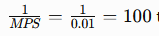 times.
Leakages or withdrawals of multiplier
Leakages are the potential diversions of the income stream that tend to weaken the multiplier effect of new investment. Saving is a major leakage of the multiplier process. The disposable income of the individual can be saved or consumed. The higher the marginal propensity to save, the smaller the size of the multiplier; hence, the greater the amount of leakage.
Importance of multiplier
The importance of multiplier in modern economics lies in the following:
Highlights the importance of change in planned savings and autonomous consumption on income and employment: Fluctuations in income and employment are due to fluctuations in the rate of investment. A change in investment leads to a cumulative change in income and employment by the multiplier process.
Important tool in the formulation of economic policies geared to investment: If investment is small, the government can design policies to promote investment because a rise in investment has a large multiplier effects on income.
Helps the government to decide upon the amount of investment to be injected into the economy. This will eventually reduce unemployment and achieve full employment level.
Helps in bringing equality between saving and investment: When there is a disequilibrium between saving and investment, an increase in investment will lead to the increase in income more than the increase in initial investment. As a result of the increase in income, saving also increases and equals investment.
Highlights the importance of deficit financing: During depression the government will adopt an expansionary fiscal policy by increasing government expenditure or by creating deficit budget. The creation of a deficit budget is financed through deficit financing which helps to increase income and employment by multiplier times the increased investment.
Exercise 2.3
1. If the MPC is 0.6, what is the value of MPS?
2. Show why the sum of MPC and MPS is equal to one.
3. Suppose as consumption function is given by C =100+0.4Y and investment function by I = 50, where C is consumption expenditure, I is investment expenditure and Y is the disposable income. Compute:
- The equilibrium level of income;
- The consumption level at equilibrium; and
- Final change in equilibrium income if change in investment is TShs 10,000.
Chapter summary
1. National income is the monetary value of all final goods and services produced in the economy by factors of production in a certain period of time, usually one year.
2. The total income in the economy must be equal to the total expenditure because in every transaction the firm receives revenue that is the same amount as spent by the households.
3. The Gross Domestic Product (GDP) measures the total expenditure on all final goods and services produced in a given period and total income earned by all factors of production participated in producing these goods and services. In simple terms, GDP is the market value of all final goods and services produced within a country in a year.
4. The GDP identity comprises of four components namely; consumption spending, investment spending, government spending, and net exports. Consumption spending includes goods and services consumed by the households. Investment spending is the purchase of intermediate goods used in the production of goods and services, and inventories by the firms. Government spending is the spending on purchasing of goods and services by government ministries, departments and agencies. Net exports include the values of goods and services produced in the domestic economy and sold outside the country (exports), minus the value of goods and services produced outside the nation's borders and sold within the economy (imports).
5. The Gross National Product (GNP) is the market value of all final goods and services produced by the citizens of a particular country in a given period of time regardless of their location. It is a GDP plus the net factor income from abroad.
6. Economists prefer to use real GDP to measure economic prosperity of a nation since the higher the real GDP, the better the well-being of the people. The nation can afford to provide good education system, affordable health services, and good transport and communication system. But GDP does not include leisure which adds to the standard of living, government spending on non-welfare improving activities, and does not show how income is distributed. Therefore, GDP is an imperfect measure of the economic welfare of a country.
7. In the national income computations, economists usually use three methods namely; the output method, the income method and the expenditure method. In the output method, the value added at each stage of production is aggregated for all goods and services produced in an economy to arrive to GDP. In the income method, the incomes earned by all factors of production are aggregated to come up with one figure. In the expenditure method, the GDP is computed by aggregating the expenditures of households on final goods and services, the expenditure of firms on intermediate goods, government purchases of goods and services and net exports. In theory, all the three methods result to the same figure of GDP. But practically, because the data are not perfect, sometimes the figures may be different.
8. The process of computing national income is not straight forward. There are some challenges which are worthwhile to mention. Some of these problems are double counting, inadequate statistical data, and non-marketable goods and services.
9. The level of national income is determined by the Aggregate Demand (AD) and the Aggregate Supply (AS). The equilibrium level of national income is determined by AD, since AS remains more or less constant in the short run. Therefore, the national output is assumed to be as much as the effective demand.
10. The effective demand is divided into two components: The demand for consumption goods by people and government in the economy and demand for intermediate goods by firms.
11. The equilibrium level of national income is determined by leakages-injections approach, whereby in the closed economy with no government sector saving is the only leakage and investment is the only injection. Thus, at equilibrium leakages must be equal to injections. That is, savings must be equal to investment. That is why the leakages-injections approach is sometimes known as the savings-investment approach.
12. The shift in aggregate expenditure leads to the changes in the equilibrium national income. For instance, if the aggregate expenditure increases (shifting upward), the equilibrium national income also increases and the vice versa is true in case of decrease in aggregate expenditure. Therefore, in the leakages-injections approach a shift in savings or investment curves leads to the changes in the equilibrium national income.
13. The relationship between change in the equilibrium national income and investment is expressed by the investment multiplier. The investment multiplier is an average number of times in which initial change in the investment multiplies several times to give the final change in the equilibrium national income.
www.learninghubtz.co.tz
Revision exercise
1. Is it true that all three approaches of computing national income result to the same figure? If it is true; why one keep using three approaches, if one approach can serve the purpose?
2. In a speech that Mwalimu Julius KambarageNyerere gave as the first president of the United Republic of Tanzania in 1964, he said the following about GDP per capita: “It does not talk about good health care of our society and better education system. It does not talk about the patriotism and trustfulness of our public officials. It does not measure our courage, our wisdom, our dedication or commitments to our country. It measures everything, except that which makes life valuable, and it can tell us everything about Tanzania except why we are proud that we are Tanzanians”. Do you think that Mwl. J. K Nyerere was right? If so, why do we care about GDP per capita?
3. According to the World Bank report, the value of GNP and GDP of Tanzania were TShs 17.35 and TShs 23.87 trillion respectively in the year 2015. Give the possible reasons why the value of GDP in Tanzania is larger than the value of GNP.
4. Assess the strengths of using national income statistics as an indicator of standards of living and for comparing economic development between different countries.
5. Consider the expenditure and income items of an economy, then answer the following questions (Figures are in billions Tanzanian shillings):
- Personal taxes . . . . . . . . . . . .40
- Social security contributions . . . . . ..15
- Indirect business taxes . . . . . . . ..20
- Corporate income taxes . . . . . . . ..40
- Transfer payments . . . . . . . . . ..22
- Tanzania exports . . . . . . . . . ..24
- Tanzania imports . . . . . . . . . ..22
- Subsidies . . . . . . . . . . . . .10
- Personal consumption expenditures . . ..255
- Gross private domestic investment . . . ..75
- Undistributed corporate profits . . . . .35
- Government purchases . . . . . . . ..95
- Depreciation (capital consumption allowances) .25
- Dividends . . . . . . . . . . . . ..2
- Net foreign factor income earned in Tanzania .10
Calculate:
- GDP factor cost using expenditure methods;
- Net domestic product;
- National income;
- Personal income; and
- Disposable income.
6. The following table shows items of the income statement of an economy for the year 2019/2020 in billions of shillings:
| Items | Amount (TShs) |
| Rent | 24 |
| Personal consumption expenditure | 1,080 |
| Corporate income taxes | 65 |
| Undistributed corporate profits | 180 |
| Net exports | 7 |
| Dividends | 35 |
| Net income from abroad | 100 |
| Capital consumption allowance/depreciation | 80 |
| Interest | 82 |
| Indirect business taxes | 101 |
| Gross private domestic investment | 240 |
| Compensation of employees | 1,028 |
| Government purchases of goods and services | 365 |
| Proprietors’ income | 97 |
- Determine the Gross Domestic Product at market price using expenditure and income approaches;
- Compute the Net Domestic Product (NDP); and
- Compute Gross National Product (GNP).
7. In 1970, the government of Tanzania increased investment spending by TShs 8 billion. Given that the Marginal Propensity to Consume (MPC) is 0.75, and assuming further that the economy was initially in the equilibrium income at TShs 500 billion:
- Its effects on the national income equilibrium;
- Assuming that instead of an increase by TShs 8 billion, there was a drop in investment by TShs 8 billion, what would happen to the national income equilibrium? and
- Why is it important for a government to consider the concept of investment multiplier when making policy decisions?

Hub App
 For Call,Sms&WhatsApp: 255769929722 / 255754805256
For Call,Sms&WhatsApp: 255769929722 / 255754805256  MATOKEO YA KIDATO CHA VI 2026
SECONDARY REGIONAL EXAMS
PRIMARY REGIONAL EXAMS
FORM VI NECTA REVIEWS
FORM IV NECTA REVIEWS
FORM II NECTA REVIEWS
STD VII NECTA REVIEWS
STD IV NECTA REVIEWS
SECONDARY EXAMS SERIES
PRIMARY EXAMS SERIES
PRIMARY SUBJECT NOTES
SECONDARY SUBJECT NOTES
SECONDARY TOPICAL EXAMS
SECONDARY TOPICAL QUESTIONS
PRIMARY TOPICAL QUESTIONS
PRACTICAL EXAMS & NOTES
SECONDARY REGIONAL EXAMS
DOWNLOAD SUBJECT NOTES
SCHEMES OF WORK (PRIMARY & SECONDARY)
LESSON PLAN
SECONDARY LOG BOOKS
PRIMARY LOG BOOKS
LITERARY WORKS / UCHAMBUZI VITABU
METHALI ZOTE ZA KISWAHILI
Vitendawili Vya Kiswahili
FORM VI RESULTS 2024
FORM FIVE SELECTION 2024
Matokeo KIDATO CHA II 2024
Matokeo Darasa IV 2024
MATOKEO KIDATO CHA IV 2023
FORM ONE SELECTION 2024
FORM VI RESULTS 2023
Matokeo Darasa IV 2022
MATOKEO YA KIDATO CHA VI 2026
SECONDARY REGIONAL EXAMS
PRIMARY REGIONAL EXAMS
FORM VI NECTA REVIEWS
FORM IV NECTA REVIEWS
FORM II NECTA REVIEWS
STD VII NECTA REVIEWS
STD IV NECTA REVIEWS
SECONDARY EXAMS SERIES
PRIMARY EXAMS SERIES
PRIMARY SUBJECT NOTES
SECONDARY SUBJECT NOTES
SECONDARY TOPICAL EXAMS
SECONDARY TOPICAL QUESTIONS
PRIMARY TOPICAL QUESTIONS
PRACTICAL EXAMS & NOTES
SECONDARY REGIONAL EXAMS
DOWNLOAD SUBJECT NOTES
SCHEMES OF WORK (PRIMARY & SECONDARY)
LESSON PLAN
SECONDARY LOG BOOKS
PRIMARY LOG BOOKS
LITERARY WORKS / UCHAMBUZI VITABU
METHALI ZOTE ZA KISWAHILI
Vitendawili Vya Kiswahili
FORM VI RESULTS 2024
FORM FIVE SELECTION 2024
Matokeo KIDATO CHA II 2024
Matokeo Darasa IV 2024
MATOKEO KIDATO CHA IV 2023
FORM ONE SELECTION 2024
FORM VI RESULTS 2023
Matokeo Darasa IV 2022
WHATSAPP US NOW FOR ANY QUERY
App Ya Learning Hub Tanzania